Section 4.1: Scatterplots and Correlation

Scatterplots

When two variables are related to each other in some way, we say they are associated. For example, Yelp ratings could be associated with Pizza chains, where certain chains tend to get higher Yelp ratings than other chains. If you knew the chain, you might be able to guess the rating for the restaurant. If you know the rating, you might be able to guess the pizza chain. That’s what we mean when we say the variables are related. Knowing one of the variables gives insight into the other variable.

Any two variables may be related, and when they are, we say there is an association. Note that an association may exist between two qualitative variables, one qualitative and one quantitative variable, or between two quantitative variables. In this chapter, we will focus on associations between paired quantitative variables. An association between paired quantitative variables is called a correlation. When we say that two variables are correlated, we are talking about numerical data. Data consisting of paired quantitative variables is called bivariate data.

When we have bivariate data, we think of them as ordered pairs, using the following definition.

We use a scatterplot, or scatter diagram, to visualize the relationship between pairs of data. A scatterplot is a two-dimensional graph containing all the data pairs plotted as points in the cartesian coordinate plane.

Solution:To make a scatterplot, we first need to create horizontal and vertical axes. We use the horizontal axis (we normally think of it as the x-axis) for the exam 1 scores, so it needs to be long enough to include scores from 0 to 95. The vertical axis we normally think of it as the y-axis) will be used for the exam 2 scores, so it will need to be long enough to include grades from 73 to 90.

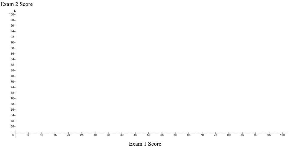
Next, we treat the exam 1 scores as the x-variable, and the exam 2 score as the y-variable to create points to add to the plot.

The first three student scores are for Derek plotted at the point (70,81), Marshawn, plotted at (95,87), and for Isabel, plotted at (80,82). For each, we drew a vertical dashed line at the x-value, and a horizontal dashed line for the y-value. The place where the dashed lines intersect is where we plot the point for that student.

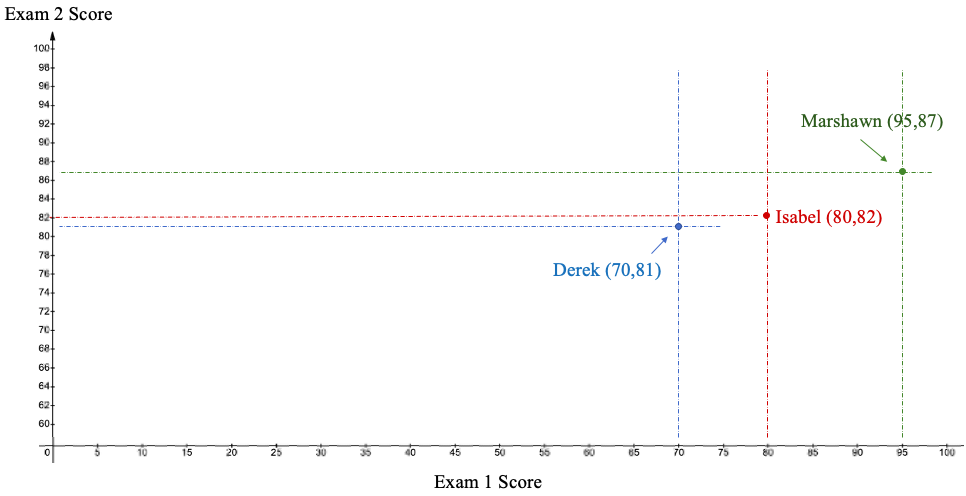
We continue in this way until all the ordered pairs are plotted as points in the scatterplot. See figure 4.2.

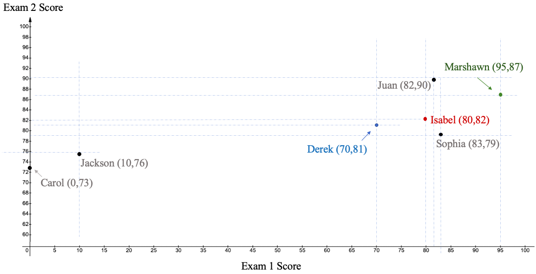
Figure 4.2: Scatterplot of exam scores.

If we remove the dashed lines and student names, we have the complete scatterplot. It appears that students who scored higher on exam 1 also tended to score higher on exam 2. Students who scored lower on exam 1 tended to score lower on exam 2. This is called a positive association between variables. Higher scores on exam 1 are associated with higher scores on exam 2. We will discuss other types of associations shortly.

Of course, drawing a scatterplot using technology is much easier and faster than doing it by hand. In this book we will primarily use STATBELT Utility- the Statistical Basics Exploratory Learning Tool (opens in a new tab), to create our scatterplots. Google Sheets will also make scatterplots.

Solution:Type or paste the data into two columns of STATBELT Utility. Paste only the numbers, and type “Exam 1 Score” and “Exam 2 Score” in the column headings. Then select Graphs → Scatterplot.

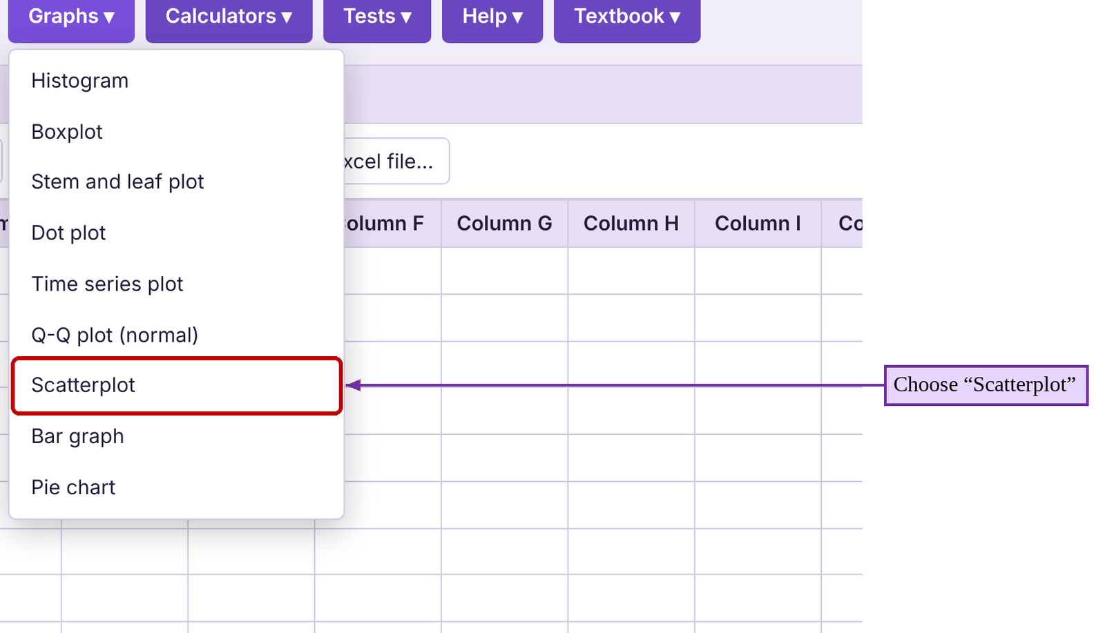
Choose “Exam 1 Score” for “Explanatory variable (x)” and “Exam 2 Score” for “Response variable (y).” Click “Open graph in a new window.” The STATBELT Utility scatterplot is shown in figure 4.3.

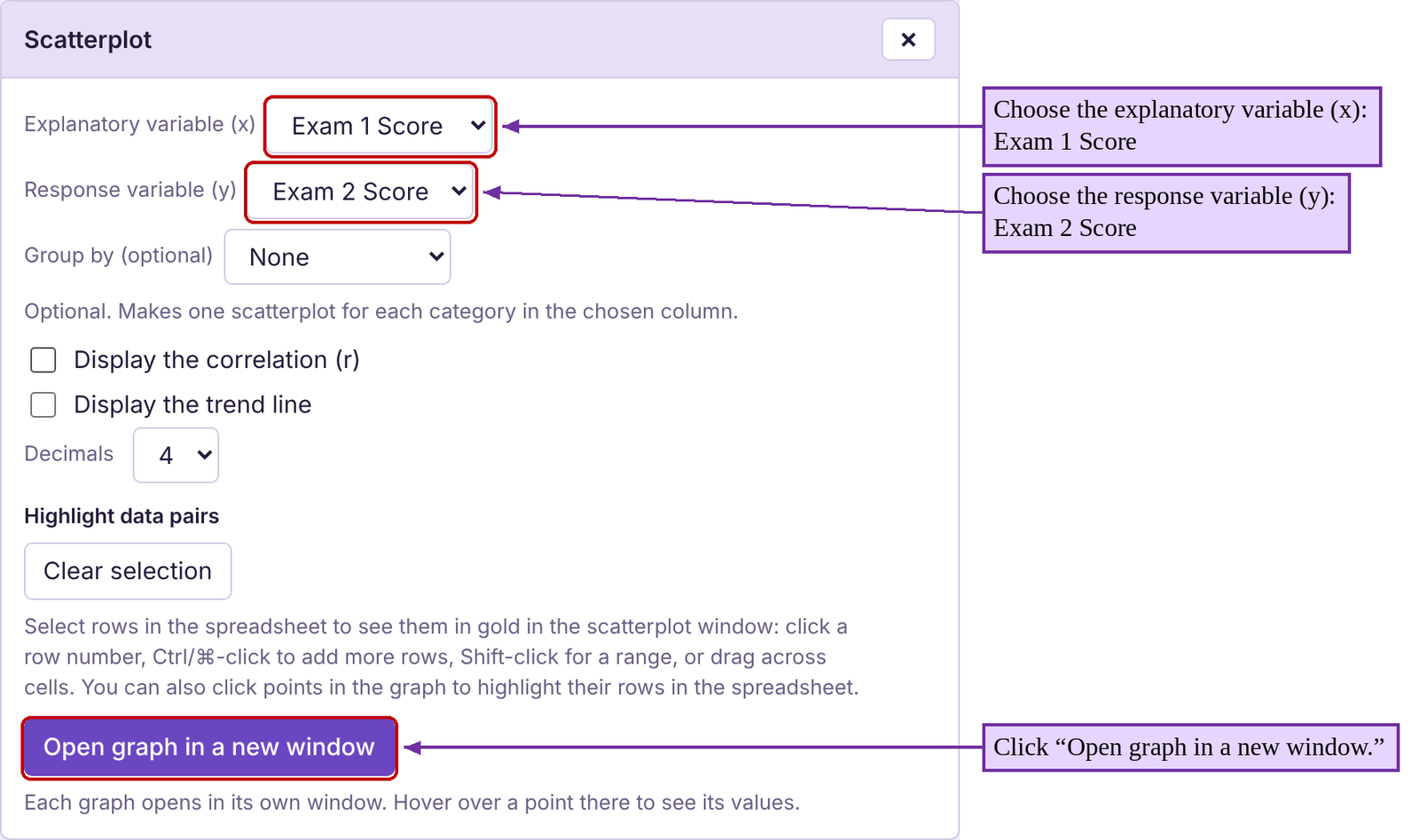
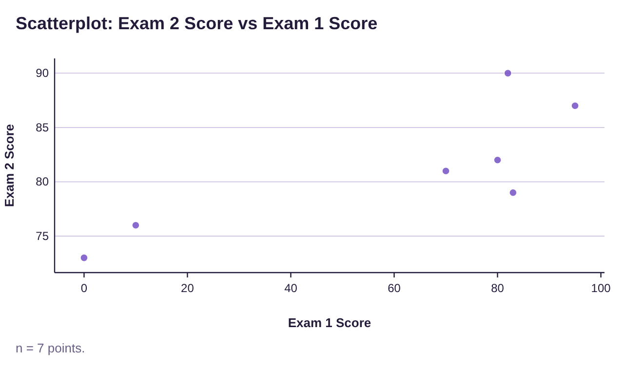
Figure 4.3: Scatterplot of exam scores by STATBELT Utility.

Again, we can see there is a trend. The explanatory variable “Exam 1 Score” gives us a hint as to what the response variable “Exam 2 Score” will be. For example, if a student scored well on the first test, you would tend to think they would score well on the second test. If they did not perform well on the first, it feels more likely that they might do poorly on the second too.

As the last example shows, we can use a scatterplot to view possible correlations between two quantitative variables. Although there are different types of correlations to view, we will look only for linear correlation in this book. Figure 4.4 shows scatterplots for the types of correlations we will see.

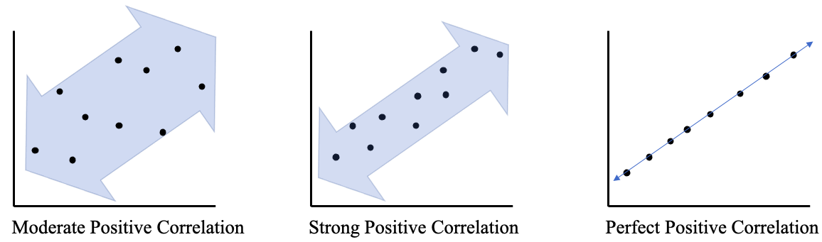
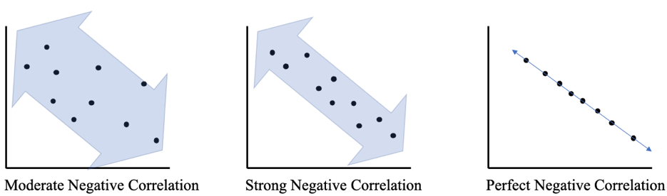
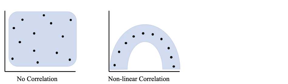
Figure 4.4: Types of Correlation and Scatterplots Chart.

Tip!

Figure 4.5: Protein vs Total Fat scatterplot for example 3.

Solution:This appears to be a strong positive correlation. Lower amounts of total fat seem to correspond with lower amounts of protein. Higher amounts of total fat appear to correspond to higher amounts of protein. If you were to draw a line through the data that shows the trend, it would have a positive slope. The points would be close to the line, indicating a strong positive correlation.

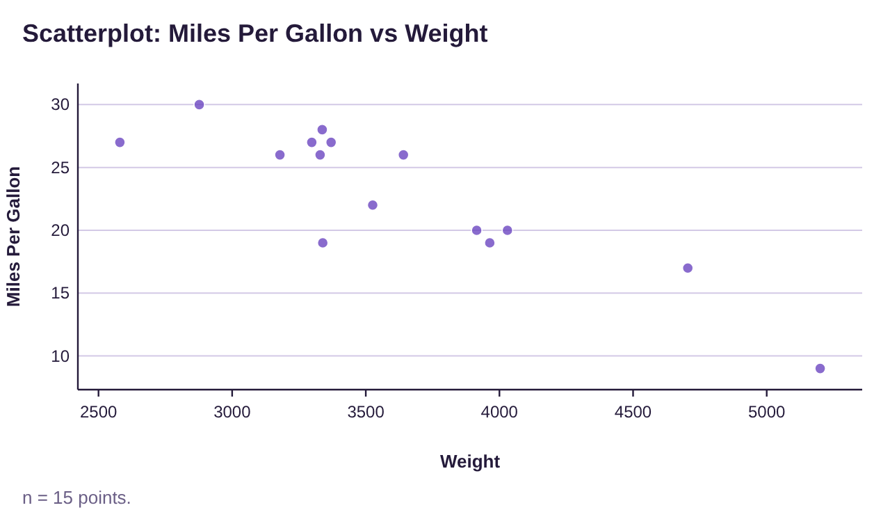
Figure 4.6: MPG vs Weight scatterplot for example 4.

Solution:This appears to be a strong negative correlation. Higher weights seem to correspond to lower gas mileage. Lower car weights appear to correspond to higher gas mileage. If you were to draw a line through the data that shows the trend, it would have a negative slope. The points would be close to the line, indicating a strong negative correlation.

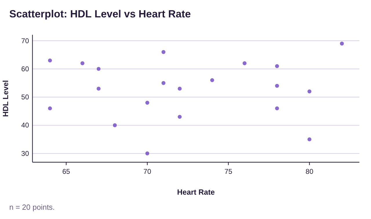
Figure 4.7: HDL cholesterol vs Heart Rate scatterplot for example 5.

Solution:There appears to be no pattern to the data at all. Having a slower or faster heart rate does not appear to have any predictive power in guessing HDL cholesterol. Knowing your cholesterol doesn’t seem to help in predicting heart rate. The data are scattered to all corners of the scatterplot, indicating that there is no correlation between these variables. Heart rate and cholesterol do not appear to be linked.

Computing Correlation as a Statistical Measure

Our next goal is to create a statistic that will measure what we see in a scatter plot. As you have probably guessed, interpreting a correlation as strong, moderate, or weak, or even if there is a correlation, is a subjective endeavor. Differences of opinions are likely to occur. For that reason, we need a numerical way to measure the linearity of the data. In other words, we want to measure “how close to a line are the points in the scatterplot?” Our statistic will need to convey this information.

The formula for linear correlation is very difficult to use by hand. It involves calculating the mean and standard deviations for the x and y variables, then the z-scores for each of the x and y data values, computing the products of the z-scores for each ordered pair, summing those products, and then dividing by one less than the sample size. Yikes! The formula was created by Karl Pearson, and is known as the Pearson Correlation Coefficient, or simply correlation. Although the formula is given, we will use technology to compute correlation in this book.

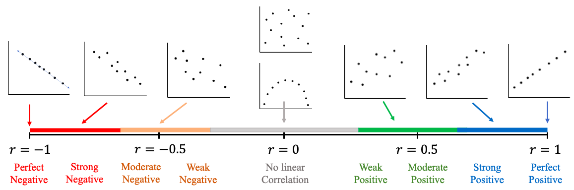
Figure 4.8: Range of correlation from -1 to +1, perfect negative to perfect positive.

Figure 4.8 shows the range of correlation you can expect to find when we calculate it using technology. The image is there to remind you how to interpret the correlation. For example, a correlation of r = -0.21 is close to 0, so it is either a very weak negative correlation or no linear correlation at all. A correlation of r = 0.75 is in the range of a moderate or strong positive linear correlation. The determination of moderate or strong to describe correlation is still subjective. It will also depend on the amount of data that has been collected. The more data you have, the more certain you can be that a correlation does or does not exist.

Solution:First, type or paste the data into two columns of STATBELT Utility and name them “Exam 1 Score” and “Exam 2 Score.” You do not need to include the students’ names. Then, select Descriptive Statistics → Correlation. Check “Exam 1 Score” and “Exam 2 Score,” then click “Show results in a new window.” The results are shown in figure 4.9.

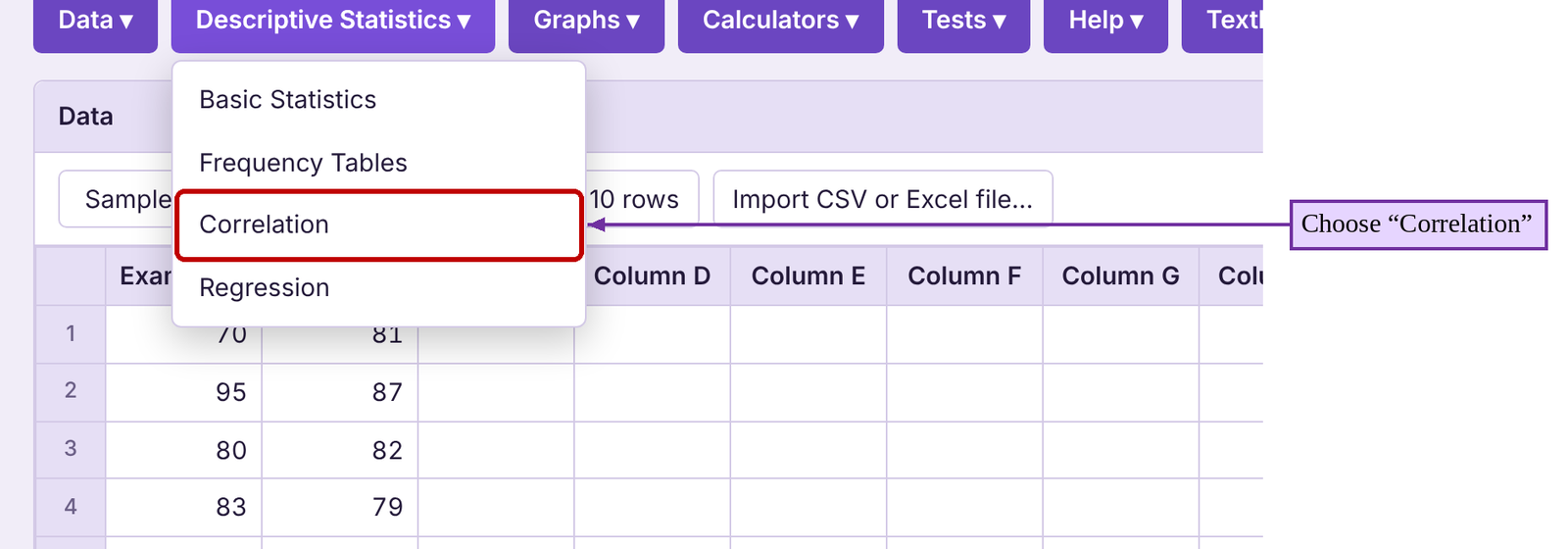
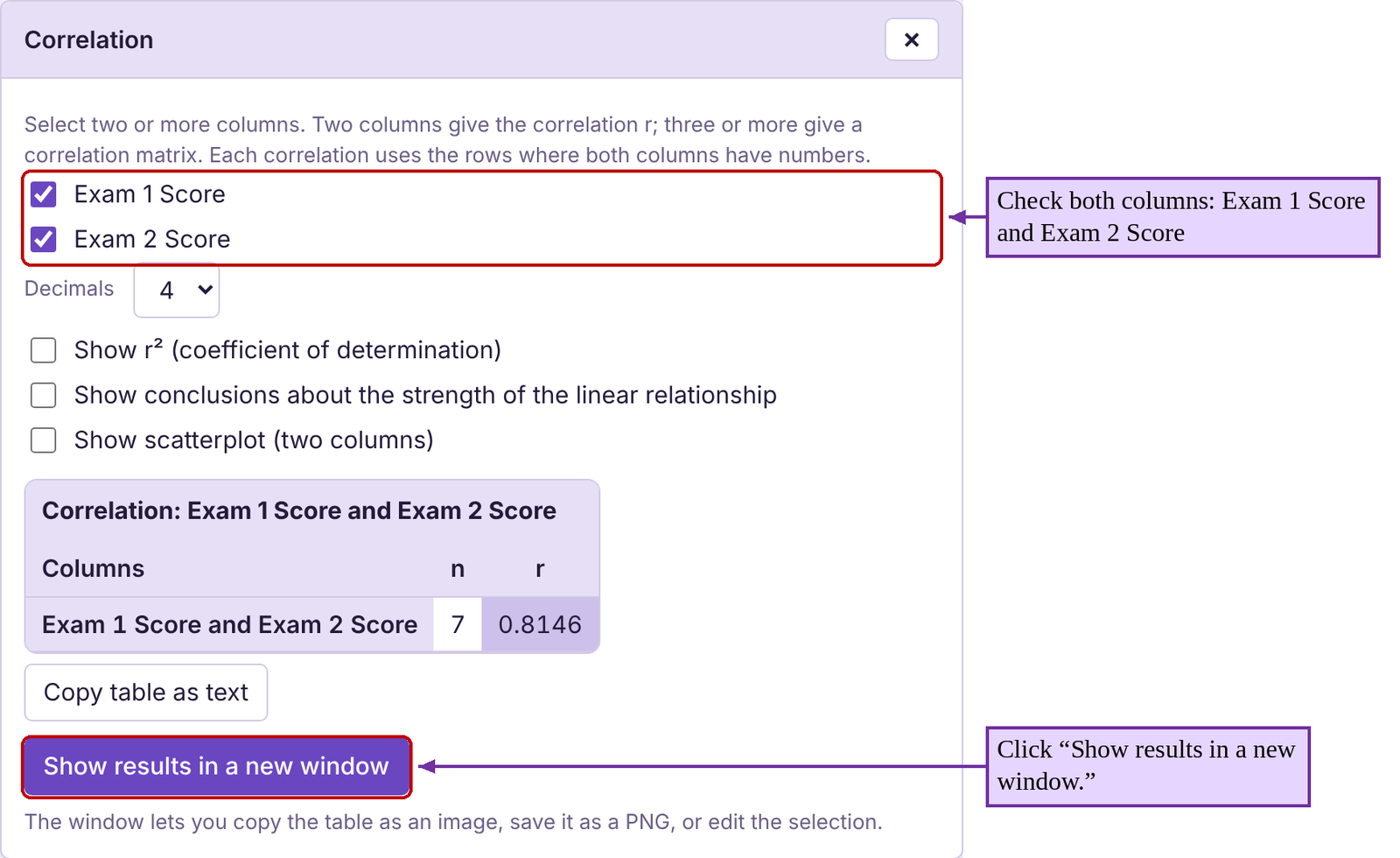
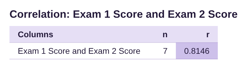
Figure 4.9: Correlation results for example 6.

The result of the correlation is r = 0.815, rounded to three decimal places. Referring to figure 4.8, this correlation is close to 1 and suggests there is a strong positive correlation, agreeing with what we noticed in the scatterplot.

Solution:To make the scatterplot, first type or paste the data into two columns of STATBELT Utility named “Total Fat” and “Protein.” Then select Graphs → Scatterplot, and choose “Total Fat” for “Explanatory variable (x)” and “Protein” for “Response variable (y).” Click “Open graph in a new window.” The scatterplot made by STATBELT Utility is shown in figure 4.10. This is the same scatterplot that was shown in example 3.

To find the correlation, select Descriptive Statistics → Correlation. Then check both “Total Fat” and “Protein,” and click “Show results in a new window.” The correlation results are shown in figure 4.10.

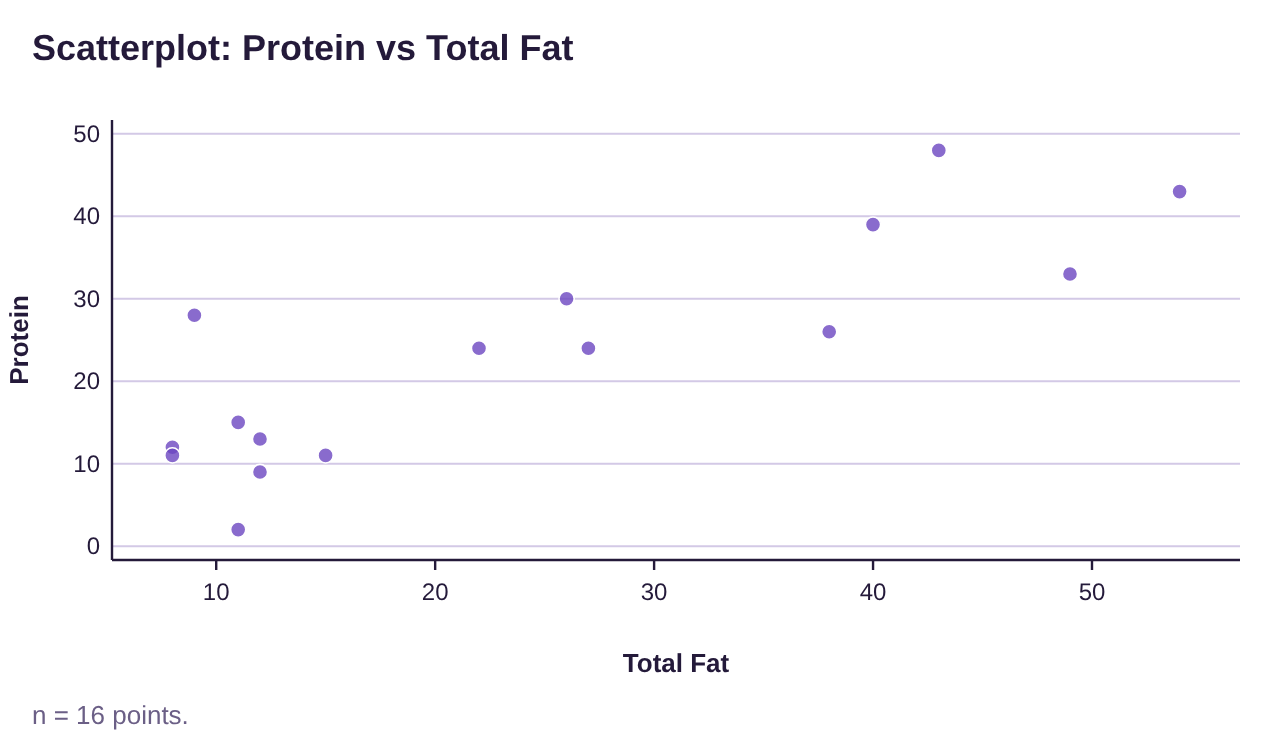
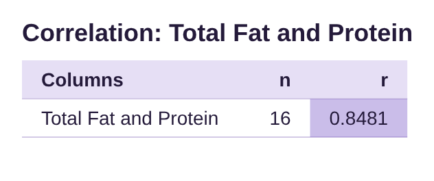
Figure 4.10: Protein vs Total Fat scatterplot and correlation.

The scatterplot shows a positive correlation. The correlation statistic is 0.848, rounded to three decimal places. This is a strong positive correlation. High total fat is strongly correlated to high protein in fast food meals.

Solution:To make the scatterplot, first type or paste the data into two columns of STATBELT Utility named “Weight” and “Miles Per Gallon.” Then select Graphs → Scatterplot, and choose “Weight” for “Explanatory variable (x)” and “Miles Per Gallon” for “Response variable (y).” Click “Open graph in a new window.” The scatterplot made by STATBELT Utility is shown in figure 4.11. This is the same scatterplot that was shown in example 4.

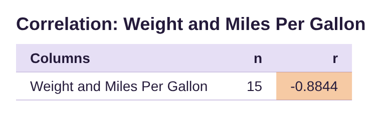
Figure 4.11: Miles Per Gallon vs Weight scatterplot and correlation.

To find the correlation, select Descriptive Statistics → Correlation. Check the columns “Weight” and “Miles Per Gallon,” and click “Show results in a new window.” The STATBELT Utility correlation output is shown in figure 4.11.

In example 4 we described this as a strong negative correlation. The correlation from STATBELT Utility is calculated as r = -0.884. Since this is negative and reasonably close to -1, the statistic agrees with our assessment of the scatterplot. If you want a car with good gas mileage, you will need to choose a lighter car. If you want a heavy car, you will have to sacrifice fuel efficiency.

Solution:We follow the same steps as the preceding examples. To make the scatterplot, first type or paste the data into two columns of STATBELT Utility named “Heart Rate” and “HDL Level.” (Table 4 lists the data in two pairs of columns, so paste the second pair under the first.) Then select Graphs → Scatterplot, and choose “Heart Rate” for “Explanatory variable (x)” and “HDL Level” for “Response variable (y).” Click “Open graph in a new window.” The scatterplot made by STATBELT Utility is shown in figure 4.12. This is the same scatterplot that was shown in example 5.

To find the correlation, select Descriptive Statistics → Correlation. Then check both “Heart Rate” and “HDL Level,” and click “Show results in a new window.” The correlation results are also shown in figure 4.12.

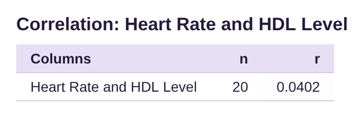
Figure 4.12: HDL cholesterol vs Heart Rate scatterplot and correlation.

In example 5 we observed that there did not appear to be any relationship between heart rate and cholesterol level. The correlation is r = 0.040, which is very close to zero. Correlations that are near zero indicate that there is no linear correlation, which agrees with what we observed in the scatterplot. Based on this data, heart rate and cholesterol do not appear to be linked.

Significant Correlation and Sample Size

At this point, we are interested in identifying when there is a “trend line” in the data that we can use to better understand the variables and make predictions. If the data follow a trend line, we will find an equation for it in section 4.2 and explore its applications in sections 4.2 and 4.3. But first we need to be able to identify and agree on when the data are following a linear pattern.

The next part of our discussion will focus on whether the data pattern is close to a line. Clearly if the correlation is very close to 1 or -1, the data are close to a line. But how close does the correlation have to be to 1 or -1 to conclude the data follow a linear pattern? This is a complicated question that will depend on two factors:

•How close the correlation r is to 1 or -1, and

•How many pairs of data are included in the sample

For a large sample of size $n=45,$ a correlation $r=0.72$ sounds like a moderate correlation. On the other hand, for a small sample of $n=7,$ the same correlation doesn’t provide the same level of certainty. Small samples are not as reliable. More data following the trend will make the trend more certain. When there is enough data to support the conclusion that there is a linear relationship between two variables, we say the correlation is statistically significant.

We use the following test to determine whether correlation is statistically significant. This is a shortcut to a more advanced topic that is sometimes included with later chapters on inference.

Table 5: Critical Values Table for Correlation

Solution:(a)We know $r=0.647$ and $n=35$ pairs of data. We locate the row for $n=35$ in the correlation table and find the critical value next to it. The critical value is 0.334.

Since $r=0.647$, $\left|r\right|=\left|0.647\right|=0.647$. And since $\left|r\right|=0.647>\mathrm{CV}=0.334$, we see that the absolute value of the correlation is larger than the Critical Value, and so we determine that the correlation is significant. The data follow a linear pattern.

(b)We are given $r=-0.412$ and $n=16$ pairs of data. We locate the row for $n=16$ in the correlation table and find the critical value next to it. The critical value is 0.497.

Since $r=-0.412$, $\left|r\right|=\left|-0.412\right|=0.412$. Here $\left|r\right|=0.412\ngtr \mathrm{CV}=0.497$. The absolute value of the correlation is NOT larger than the Critical Value, so we determine that the correlation is NOT significant. The data do not follow a linear pattern.

(c)For $n=28$ pairs of data, we locate the row for $n=28$ in the correlation table and find the critical value next to it. The critical value is 0.374.

Since $r=-0.581$, $\left|r\right|=\left|-0.581\right|=0.581$. In this example, $\left|r\right|=0.581>\mathrm{CV}=0.374$. The absolute value of the correlation is larger than the Critical Value, indicating that the correlation is significant. The data follow a linear pattern.

(d)For $n=5$ pairs of data, we locate the row for $n=5$ in the correlation table and find the critical value next to it. The critical value is 0.878.

Since $r=-0.871$, $\left|r\right|=\left|-0.871\right|=0.871$. Here the absolute value of the correlation is NOT larger than the Critical Value. In symbols, $\left|r\right|=0.871\ngtr \mathrm{CV}=0.878$, so we determine that the correlation is NOT significant. The data do not follow a linear pattern.

Note that in part (d), the correlation is not significant, even though $r=-0.871$ is close to -1. Compare that to part (a) where the correlation was considered significant with $r=0.647$, which is not as close to 1 as -0.871 is to -1. You might think that the correlation in part (d) is stronger, but that is not the case. Part (a) has much more evidence of a linear relationship because it has many more data pairs. If we want to find evidence of a linear relationship in part (d), we need to collect more data. The threshold to establish linearity decreases as the number of data pairs increases.

Putting it all Together

Finally, we will return to the first four examples of this section to interpret the data using scatterplots, correlation, and significance.

Solution:In examples 1, 2, and 6 we created the following scatterplot and computed the correlation shown in figure 4.13. There were only n = 7 students, so the critical value is CV = 0.754. The correlation is $r\approx 0.815$, and $\left|0.185\right|=0.815>0.754,$ so the correlation is significant. The scatterplot appeared to show a moderate positive correlation and now we have verified that the data do indeed follow a linear pattern.

Figure 4.13: Exam 1 and 2 scores scatterplot and correlation.

Solution:In example 3 and 7 we created the scatterplot and calculated the correlation as seen in figure 4.14.

Figure 4.14: Protein vs Total Fat scatterplot and correlation.

Based on the scatter plot, it appears that total fat and protein are positively correlated. Computing the correlation using STATBELT Utility, we obtained $r\approx 0.848$, which is a strong positive correlation (it is close to 1).

In this data set, there are n = 16 ordered pairs (the same as the number of points in the scatterplot). The critical value for n = 16 is CV = 0.497. Since $\left|r\right|=0.848>\mathrm{CV}=0.497$, we determine that the correlation is significant. The data follow a linear pattern. In fact, based on the value of r being close to 1, we would say there is a moderate to strong positive linear correlation.

Solution:We created the scatterplot and calculated correlation in examples 4 and 8, with the results below in figure 4.15.

Figure 4.15: Miles Per Gallon vs Weight scatterplot and correlation.

The scatter plot shows a negative correlation between the weight of a car and the gas mileage it gets (the data go down from left to right). STATBELT Utility confirms our suspicion. The correlation is

$r\approx -0.884$, which is close to -1.

This sample had $n=15$ pairs of data, so the critical value is 0.514. Since

$\left|r\right|=0.884>\mathrm{CV}=0.514$, we determine that the correlation is significant. The data follow a linear pattern. In fact, based on the value of r being close to -1, we would say there is a strong negative linear correlation.

Solution:We created the scatterplot and calculated correlation in examples 5 and 9, with the results below in figure 4.16.

Figure 4.16: HDL cholesterol vs Heart Rate scatterplot and correlation.

Since this correlation is $r\approx 0.04$ which is very close to 0, we suspect that there is no linear relationship.

This sample had $n=20$ pairs of data, so the critical value is 0.444. Since $\left|r\right|=0.040$ is NOT greater than the critical value 0.444, we determine that the correlation is NOT significant. The data do not follow a linear pattern, which supports the visual evidence we see in the scatter plot.

Correlation and Causation

When a correlation exists between two quantitative variables, we know that they are related. However, we must be careful not to assume that one factor is causing the other. For example, we can show that the unemployment rates for Black and White Americans from 1990 to 2020 is positively correlated with $r\approx 0.919$. That means that when the unemployment rate for one group is high, so is the other. When unemployment is lower for one it tends to be lower for the other. It does NOT mean that one of the unemployment rates is causing the other. There are underlying factors in the economy, or lurking variables, that are causing both to rise and fall together. See figure 4.17.

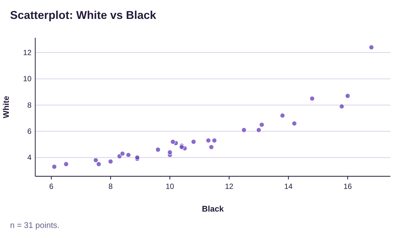
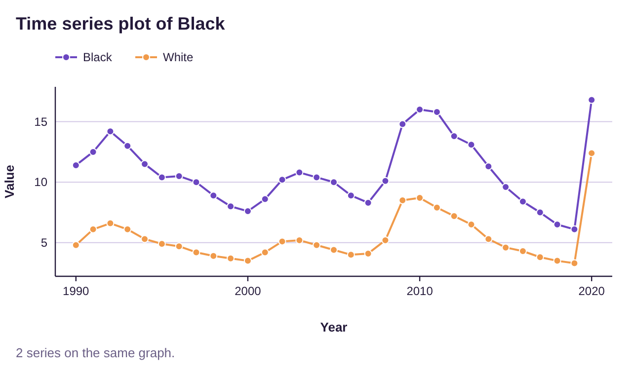
Figure 4.17: Scatterplot and time-series plot for Black and White Unemployment Rates 1990-2020.

$$\begin{array}{cc}& r\approx 0.947\end{array}$$

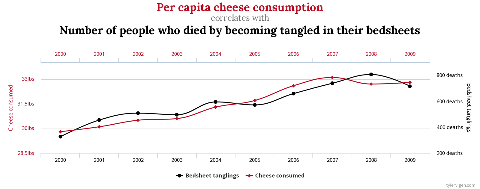
Sources: U.S. Department of Agriculture and Center for Disease Control & Prevention

It seems clear that bedsheet tangling deaths do not cause cheese consumption to increase, and that increasing cheese consumption does not cause more widespread bedsheet related death. These are likely correlated due to some underlying factor, or just plain luck. It could be an odd coincidence that as cheese consumption increased, there were more deaths due to odd circumstances, like bedsheet tangling. Whatever the reason, both were rising from 2000 to 2009. But neither caused the other to increase!

$$\begin{array}{cc}& r\approx 0.952\end{array}$$

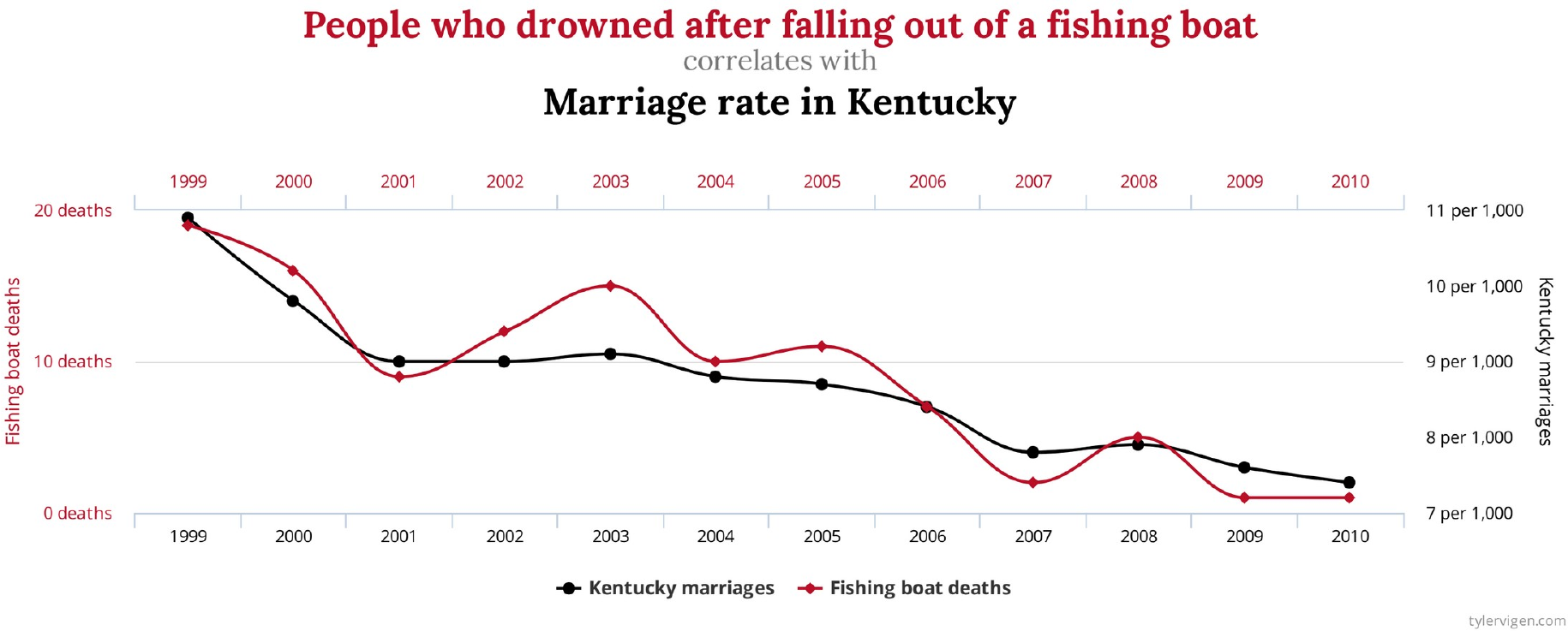
Sources: National Vital Statistics Reports and Center for Disease Control & Prevention

We aren’t even going to try to explain this graph. Please just remember that correlation does not imply causation!