Section 4.3: Residuals and Explained Variation

The Scope of the Least-Squares Regression Model

In section 4.2 we saw an example where the y-intercept of the least-squares regression line did not have a meaningful interpretation. In that example, we used the weight of a car in pounds as the explanatory variable x, and the fuel efficiency in miles per gallon (MPG) as the response variable y. The y-intercept would have occurred when the weight of a car was zero pounds. At that time, we mentioned that that was not possible, and we did not interpret the intercept for that reason. But what weights can we use for x in the equation? Can we use the equation to predict fuel efficiency for cars that weigh 1,500 pounds? What about cars that weigh 10,000 pounds? It makes intuitive sense that there should be limitations on how heavy or light a car could be for the equation to be useful.

It turns out that the answer to this question is not difficult. In practice, you can use the least-squares regression equation to make predictions for values that are in the range of the values where you collected the data, and the model should not be used to make predictions for values that are outside of the range of data you have.

As we saw in section 4.2, the regression line can only be used as a model when there is a significant correlation between the variables. Now, we add that it can only make useful predictions for x-values between the minimum and maximum x-values from the sample data (or data values that are very close). Sometimes relationships between variables can appear to be linear where you collected data but be non-linear outside of that range.

Think of this example: If you conduct a survey in Boise, Idaho, the results may be useful in making predictions in Boise, but not useful at all in making predictions outside of Boise. We cannot use those results to make a prediction about San Francisco, CA, for example. If we want to make predictions about San Francisco, we need to collect data there. The same is true for numerical measurements. If I only collect data from people between the ages of 20 and 30, I can’t use the results to make predictions for children, or for people in their 70’s. COVID vaccines were rolled out this way. They were first approved for adults, then later for children. Why? The pharmaceutical companies collected data on adults first and were able to make predictions about the efficacy of the vaccines based on that data. Later, they collected data on children and showed the vaccines were safe and effective for that population as well.

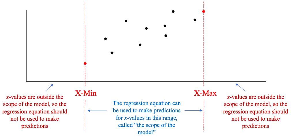
Figure 4.29: The scope of the least-squares regression model.

Solution:The smallest x-value in the data is 8, and the largest x-value in the data is 54. So here, X-Min = 8 and X-Max = 54. The model should make a reasonable prediction for any x-values between 8 and 54 grams of total fat. Thus, the model should not be used for x = 0 grams of total fat, nor for x = 100 grams of total fat. Both 0 and 100 are outside the scope of the model, so we make no predictions using these values. We can use the model to predict protein for x = 40 grams of total fat because it is between 8 and 54.

The predicted amount of protein for x = 40 grams of total fat is

$$\begin{array}{cc}\widehat{y}& =5.9+0.71x\\ \widehat{y}& =5.9+0.71\left(40\right)\\ \widehat{y}& =5.9+28.4\\ \widehat{y}& =34.3\end{array}$$

This means fast food meals containing 40 grams of total fat will have 34.3 grams of protein, on average.

Now, in the last example, it would seem reasonable to use the model to predict protein for total fat values that were near X-Min and X-Max, even if they were outside the scope of the model. How far below X-Min = 8 or how far above X-Max = 54 you can go and get reliable results is subjective. For example, we could probably trust the model if we used it to predict protein for x = 6 (very close to X-Min =8) or x = 55 (very close to X-Max -54). As a guide, you can probably extend the scope of the model by 5 to 10% of the range of x-values both below X-Min and above X-Max, assuming the values make sense in the context of the variables. For the last example, the range of x-values is Range = 54 – 8 = 46. Five percent of 46 is $0.05\times 46=2.3$ and ten percent of 46 is $0.10\times 46=4.6$, so you can probably trust the model to go two to four points lower than 8 and two to four points higher than 54. So, we can extend the model to make predictions from around 4 or 5 grams of total fat up to around 57 or 58 grams of total fat. The farther you extend outside the scope, the more likely the prediction you make will be wrong. So, you should always be careful making predictions outside the range of your data collection!

Residuals

When we use a regression line to model the linear trend, it is most often the case that the line does not pass through all the data the points. The points in the data set will be closer to the line when the correlation is strong and be farther from the line when the correlation is weak. A residual is a measure of how different a particular data value is from the predicted value found using the least-squares regression line.

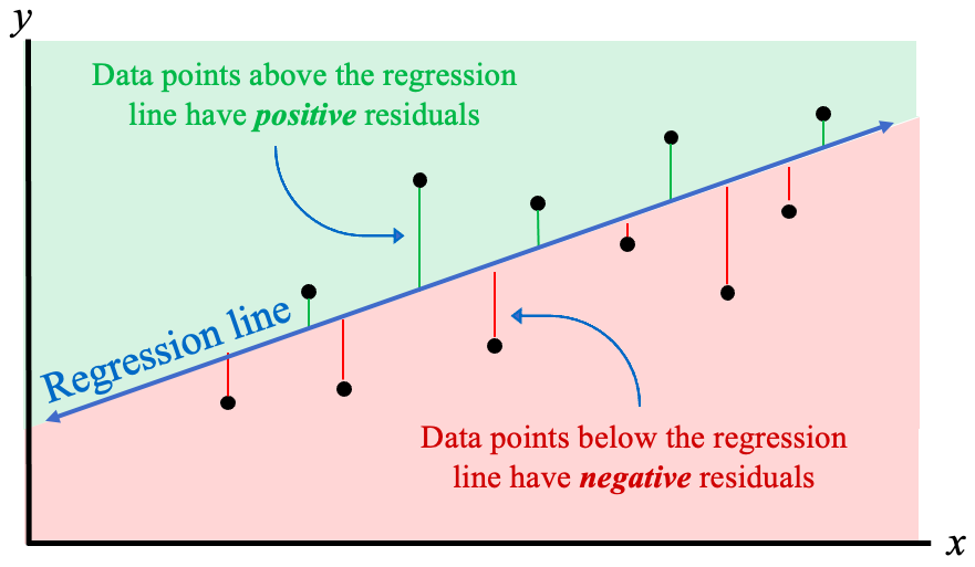
Figure 4.30: The residuals are the signed distances from the data points to the regression line.

The least squares regression line is the line that makes the sum of the squares of the residuals as small as possible (that is where the term “least-squares” comes from). Fortunately, we are using technology to compute the line, but we will still use residuals to measure data values against the predicted value from the regression equation. The sum of the squared residuals is also called the “unexplained variation” for reasons we will discuss later.

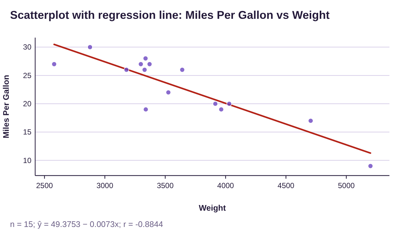
Figure 4.31: Miles Per Gallon vs Weight scatterplot and least-squares regression line.

Solution:(a)To predict the MPG for a car that weighs 3339 pounds, plug $x=3339$ into the equation.

$$\begin{array}{cc}\widehat{y}& =49.4-0.0073x\\ \widehat{y}& =49.4-0.0073\left(3339\right)\\ \widehat{y}& =49.4-24.3747\\ \widehat{y}& \approx 25.0\end{array}$$

So, cars that weigh 3339 pounds are expected to get about 25.0 MPG, on average.

(b)The residual is $\text{Residual}=\text{Observed}y-\text{Predicted}y=y-\widehat{y}$. The observed mileage is 19, and the predicted mileage is 25.0, so the residual is

$$\begin{array}{cc}& \text{Residual}=19-25.0=-6.0\mathrm{.}\end{array}$$

(c)Since the Chevy Camaro from the data set gets 19 MPG, we can see that it performs worse than the predicted mileage of 25.0 MPG. The residual = – 6.0 tells us how much worse than predicted. The interpretation is that the Chevy Camaro gets 6 MPG less than the average of cars of the same weight. The phrase “less than” takes the place of the negative sign in the residual. You can visualize the residual as the length of the purple line segment connecting the regression line to the point representing the Camaro below it in figure 4.32. Of course, people don’t purchase a Camaro to get good gas mileage!

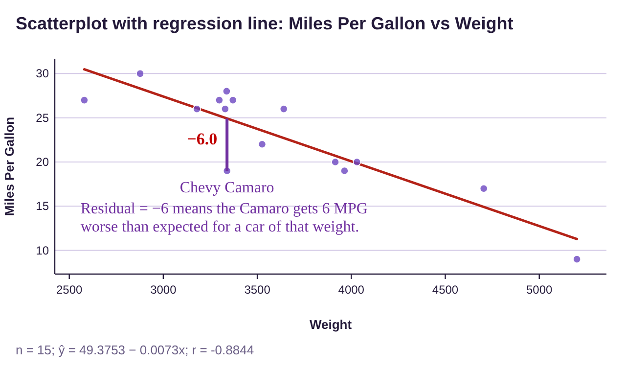
Figure 4.32: Miles Per Gallon vs Weight with the Chevy Camaro residual.

Solution:The residual is the observed mileage of a Subaru Outback (26 MPG) minus the predicted mileage for cars that weigh 3641 pounds (the weight of the Outback). First, we find the predicted mileage by substituting x = 3641 into the regression equation.

$$\begin{array}{cc}\widehat{y}& =49.4-0.0073x\\ \widehat{y}& =49.4-0.0073\left(3641\right)\\ \widehat{y}& =49.4-26.5793\\ \widehat{y}& \approx 22.8\end{array}$$

So, cars that weigh the same as a Subaru Outback will average about 22.8 miles per gallon. Next, the residual is

$\text{Residual}=\text{Observed}y-\text{Predicted}y=26-22.8=3.2$. The interpretation of the residual is that the Subaru Outback gets about 3.2 MPG higher than the average for cars of that weight. The residual is positive, indicating that the point representing the Subaru Outback is above the regression line. See figure 4.33.

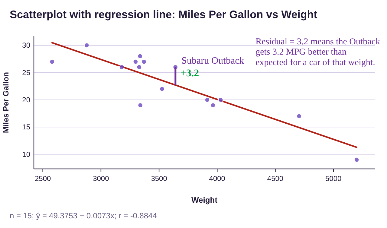
Figure 4.33: Miles Per Gallon vs Weight with the Subaru Outback residual.

Explained Variation

When you consider the scatter plot for weights of cars and gas mileage from the previous two examples, you can see that few of the data points are on the least-squares regression line. Data points that are on the line are exactly where we expect them to be using the weight as a predictor. In that sense, the model has explained them. Data points that are not on the regression line are not where they were predicted to be and have what we call unexplained deviations. The unexplained deviation comes from factors other than the weight of the car. Fuel efficiency is also impacted by aerodynamics and engine size, for example. So, the weight of a car only partially explains the gas mileage it will get. Our next goal is to find a way to describe how large of a factor the weight is in predicting the gas mileage.

As an example of explained and unexplained variation, consider your paychecks for working an hourly job. Assume you are paid $20 per hour. The variation in your paycheck will be due to the number of hours that you work. Weeks you work fewer hours will result in smaller paychecks. Weeks when you work more hours will result in larger paychecks. The differences in your paychecks are called “explained variations” because the number of hours you work will “explain” the amount of pay. Now, if you work on a commission as well as hourly pay, the variation in your paycheck is due to not only the hours worked (the explained variation), but also by the number and size of commissions. The amount of pay that comes from commissions is not explained by the number of hours worked so it is called “unexplained variation.” You can think of explained variation as the variation that is accounted for by the x-variable. Unexplained variation is the any further variation. The total variation is the sum of the explained variation (from the regression model) and the unexplained variation (the left-over).

The coefficient of determination is the ratio of explained variation to total variation, or simply the proportion of explained variation. The derivation of the idea is complicated, but the interpretation is useful and not very difficult to understand. To create the formula, the total variation is calculated using the mean of all the y-values in the data, $\bar{y}$. The total deviation for one observation is the difference between the observed y-value and the mean $\bar{y}$, ($\bar{y}$ is indicated by the horizontal line in figure 4.34). The total deviation can be divided into two parts, the part that is explained by the linear model (the blue segment which shows the vertical distance between the mean and the regression line in figure 4.34), and the residual that is not explained by the linear model (the red segment which shows the vertical distance between the data value and the regression line).

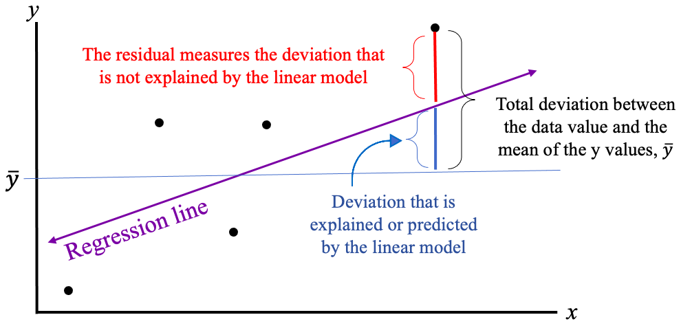
Figure 4.34: Total deviation, explained deviation, and unexplained deviation.

It is outside the scope of our discussion to prove that the sum of the squared residuals is the unexplained variation, and that the remainder of the total of the squared total deviations is the explained variation. The derivation of the formula looks very similar to deriving the standard deviation formula, but again, we will use technology to compute it. We only ask that you remember that residuals measure the unexplained deviations that lead us to the coefficient of determination.

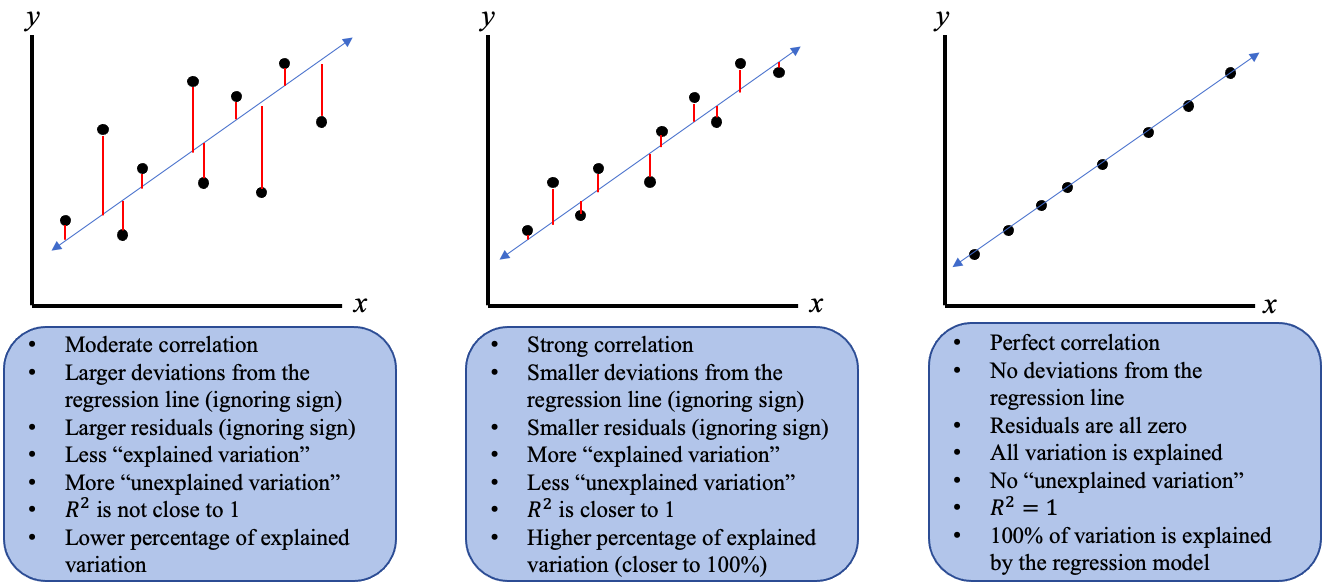
Figure 4.35: Interpretation of the coefficient of determination.

When the data are scattered far from the least-squares regression line, there is a weaker correlation, the residuals are larger in magnitude, and less of the variation is explained by the model. When the data are closer to the least-squares regression line, there is a stronger correlation, the residuals are smaller in magnitude, and more of the variation is explained by the model. If there is a perfect correlation, the model explains 100% of the variation.

Tip!

Solution:Since we are given the correlation, we can use the formula $R^2={\left(r\right)}^2$. Using a calculator, we get the coefficient of determination is $R^2={\left(r\right)}^2={\left(0.81458\right)}^2\approx 0.6635$. This means that approximately 66.35% of the variation in the exam 2 scores is explained by the exam 1 score. Note that 100 – 66.35 = 33.65% is unexplained by the exam 1 score. So, the least-squares regression line does a good job of identifying a trend, capturing 66.35% of the variation, but the predictions it gives are not very precise. The unexplained 33.65% of variation is more than a 3-letter grade difference!

Solution:We have two options. We could calculate the correlation using Descriptive Statistics → Correlation. Check both variables, then click “Show results in a new window.” Then we could use a calculator to square the correlation to find $R^2$.

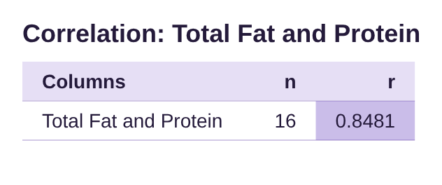
The coefficient of determination is $R^2={\left(r\right)}^2={\left(0.84807168\right)}^2\approx 0.719$.

Alternatively, we could use Descriptive Statistics → Regression. Choose “Total Fat” for “Explanatory variable (x)” and “Protein” for “Response variable (y),” then click “Show results in a new window.”

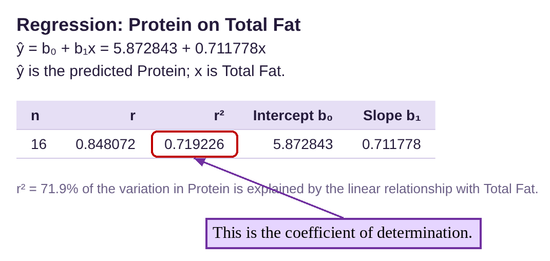
Either way, the coefficient of determination is 0.719. To interpret it, we multiply it by 100 to make it a percent. That gives us $100\times 0.719=71.9\%$. We interpret this as 71.9% of the variation in protein is explained by the fat content.

Keep in mind that there are other factors besides fat content that make up the remaining 100 – 71.9 = 28.1% of the variation in protein. For example, is the meal made with a lean source of protein, such as beans or chicken? Or is the meal fried with lots of cheese? It is also important to keep in mind that the total fat is not causing the protein to be high or low. These variables are correlated, so knowing one gives insight into the other. How much insight? About 71.9% of protein content is accounted for by knowing the fat content (not caused by it!) That’s a good measure of the predictive power of the model.

Solution:With the data in two columns in STATBELT Utility, select Descriptive Statistics → Correlation, and check both columns.

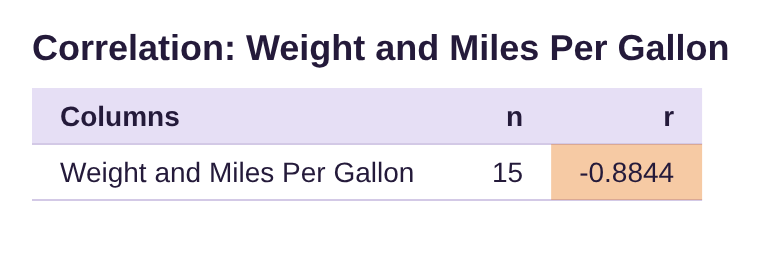
The coefficient of determination is $R^2={\left(r\right)}^2={\left(-0.88435876\right)}^2\approx 0.782$. Note that squaring the negative correlation gives a positive number!

Alternately, you can select Descriptive Statistics → Regression, then choose Weight for “Explanatory variable (x)” and Miles Per Gallon for “Response variable (y)” and click “Show results in a new window.”

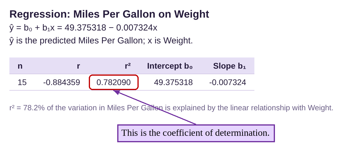
So, $100\times 0.782=78.2\%$ of the variation in miles per gallon is explained by the weight of the car. Again, the fuel efficiency is not caused exclusively by the weight, although it does seem reasonable to conclude that, in this case, higher weights should cause worse mileage. But there remains 100 – 78.2 = 21.8% of gas mileage that is caused by other factors, like engine size, design, etc. But clearly the weight of the car is an important factor in determining the fuel efficiency, accounting for 78.2%of the total variation.

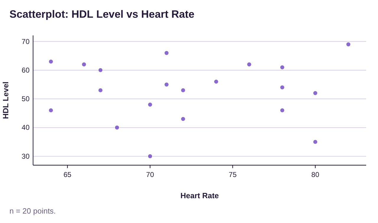
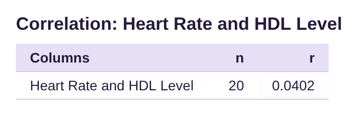
Figure 4.36: HDL cholesterol vs Heart Rate scatterplot and correlation.

Solution:The coefficient of determination is $R^2={\left(r\right)}^2={\left(0.040196208\right)}^2\approx 0.0016$. So,

$100\times 0.0016=0.16\%$ of the variation in HDL cholesterol level is explained by heart rate. This means that heart rate explains less than 1% of HDL cholesterol level, and over 99% is explained by other factors. Recall that the correlation between heart rate and HDL cholesterol level is not significant, which is consistent with heart rate explaining close to nothing about HDL cholesterol. Since the two variables are not correlated, knowing one tells you very little about the other.