Section 6.1: Discrete Random Variables

Random Variables

In chapter 1 we discussed qualitative and quantitative variables. As you may recall, quantitative variables can be categorized as discrete, or continuous. Typically, we will use discrete variables when we count something, and continuous variables are used when we measure something. In chapter 6 we will focus on discrete variables.

We will study discrete random variables in chapter 6 and continuous random variables in chapter 7. It is important to be able to distinguish between the two types of variables.

Solution:a)Since you are counting the faces and adding them, the sum is discrete. That makes the sum of two dice a discrete random variable.

b)Since you count the number of times tails shows up in the 10 coin flips, X is a discrete random variable.

c)The weight of a peanut butter cup is a measure, so X is a continuous random variable.

d)The number of spam calls received in a day is a count, so X is a discrete random variable.

e)A length of time is a measurement, so this is a continuous random variable.

f)The number of students who show up is a count, so X is a discrete random variable.

Discrete Probability Distributions

Recall that a probability distribution is a list of each possible outcome in an experiment along with its probability.

Solution:Theoretically, we can use tree diagrams to create the sample space for all the outcomes of flipping a coin 4 times. In section 5.1 example 3, we created the sample space for flipping a coin three times. We will add one more branch to create a sample space of 16 possible outcomes, shown in figure 6.1.

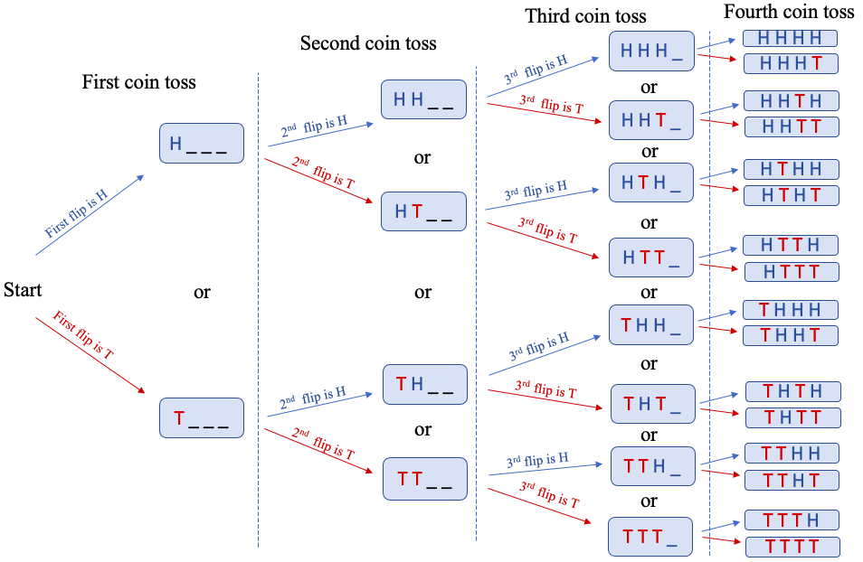
Figure 6.1: Tree diagram for 4 coin tosses.

The 16 possible outcomes are shown in figure 6.2.

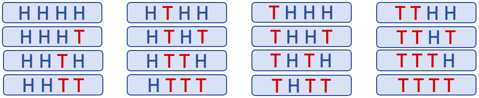
Figure 6.2: Possible outcomes of 4 coin tosses.

If we organize the sample space by the number of times tails occurred, we can calculate the probabilities needed for the probability distribution, shown in figure 6.3. There is only one way that no tails occur, so the probability that $X=0$ is $\frac{1}{16}$. There are 4 different ways where one tail occurs, so the probability that $X=1$ is $\frac{4}{16}$. The rest of the probabilities are computed in the same way.

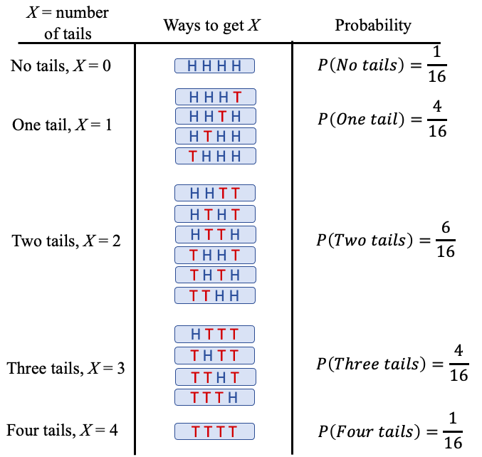
Figure 6.3: Organized samples space for counting the number of tails.

The probability distribution for DRV X = the number of tails in 4 coin flips is given in Table 1. Each of the fractions shown in figure 6.3 have been expressed as a decimal rounded to 4 places.

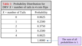
Table 1: Probability Distribution for DRV X = number of tails in 4 coin flips
X = number of Tails	Probability
0	0.0625
1	0.2500
2	0.3750
3	0.2500
4	0.0625
	1.0000

Note that each of the numbers listed in the probability column are between 0 and 1, and that the sum of all the probabilities is equal to 1. The column for X lists the number of tails you might get out of 4 coin flips, which could be any whole number between 0 and 4.

Once we have a probability distribution, we can use it to find probability. The next example could have been done in chapter 5, but the notation is new and might be a little confusing at first.

Solution:a)Using the table, $P\left(X=2\right)=0.3750$. The notation is odd because of the equality inside the probability statement. It means that “the probability that there are two tails is equal to 0.375.”

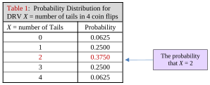
Table 1: Probability Distribution for DRV X = number of tails in 4 coin flips
X = number of Tails	Probability
0	0.0625
1	0.2500
2	0.3750
3	0.2500
4	0.0625

b)The probability that X is greater than or equal to 2 means that X is 2, or 3, or 4. As in chapter 5, the word “or” in probability tells us to add. So, we have

$$\begin{array}{cc}P\left(X\ge 2\right)& =P\left(X=2\right)+P\left(X=3\right)+P\left(X=4\right)\\ & =0.3750+0.2500+0.0625\\ & =0.6875\end{array}$$

c)Obtaining fewer than 4 tails means that 0, 1, 2, or 3 tails occurred in the four coin flips. We can either add up those probabilities, or perhaps more easily, use the complement.

$$\begin{array}{cc}P\left(X<4\right)& =1-P\left(X=4\right)\\ & =1-0.0625\\ & =0.9375\end{array}$$

About 93.75% of the time, you will get fewer than 4 tails when you flip a coin 4 times.

d)The highest probability for any of the outcomes is 0.3750. So, it appears that getting tails twice out of 4 times is the most common occurrence, happening about 37.5% of the time. Of course, there is a 50% chance of tails on any coin flip, so obtaining two tails out of four coin flips sounds reasonable.

When we work with probability distributions, we can find complicated probabilities by addition or using complements, as we did in example 3. Table 2 is a summary of phrasing you may see and the symbolic equivalent using inequalities and the variable X.

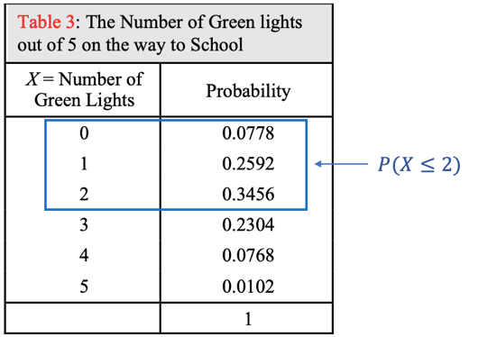
Solution:a)“At most 2 green lights” means $X\le 2$.

So, $P\left(X\le 2\right)=0.0778+0.2592+0.3456$

$$\begin{array}{cc}& =0.6826\end{array}$$

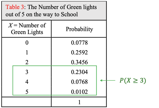
b)“At least 3 green lights” means $X\ge 3$.

So, $P\left(X\ge 3\right)=0.2304+0.0768+0.0102$

$$\begin{array}{cc}& =0.3174\end{array}$$

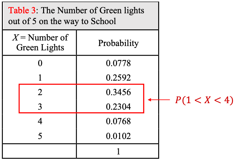
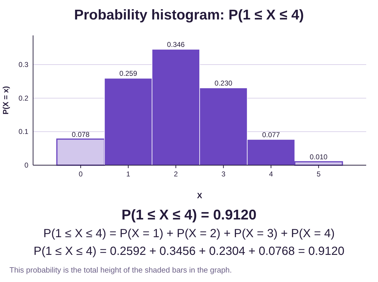
c)“Between 1 and 4 green lights, exclusive” means $1<X<4$. So, $P\left(X=1\right)$ and $P\left(X=4\right)$ are NOT included in the sum, only $P\left(X=2\right)$ and $P\left(X=3\right)$

$$\begin{array}{cc}P\left(1<X<4\right)& =P\left(2\le X\le 3\right)\end{array}$$

$$\begin{array}{cc}& =0.3456+0.2304\\ & =0.5760\end{array}$$

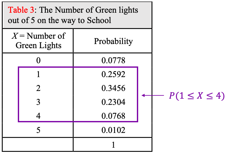
d)“Between 1 and 4 green lights, inclusive” means $1\le X\le 4$. So, $P\left(X=1\right)$ and $P\left(X=4\right)$ ARE included in the sum. The word “inclusive” tells us to include the end of the intervals.

$$\begin{array}{cc}P\left(1\le X\le 4\right)& =0.2592+0.3456+0.2304\end{array}$$

$$\begin{array}{cc}& +0.0768\\ & =0.9120\end{array}$$

You could also have computed this using the complement by subtracting the probability of

X = 0 and X = 5.

$$\begin{array}{cc}P\left(1\le X\le 4\right)& =1-0.0778-0.0102\\ & =0.9120\end{array}$$

In chapter 2 we used relative frequency tables to create relative frequency histograms. We will treat a probability distribution for a discrete random variable the same way. Once we create the probability histogram, we can use it to describe the shape of the probability distribution.

Solution:We start by marking off the horizontal X axis with the discrete numbers 0, 1, 2, 3, and 4.

Next, we add a vertical axis scaled so that the largest probability, 0.375, will be near the top of the probability histogram. In this case, we used a maximum of 0.4. Finally, we add in bars using the probability for the height of each bar. See figure 6.4.

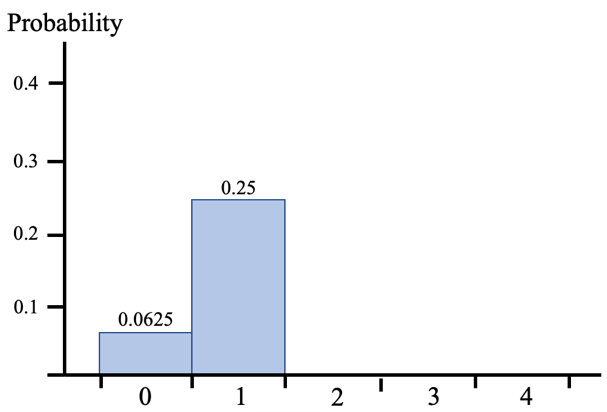
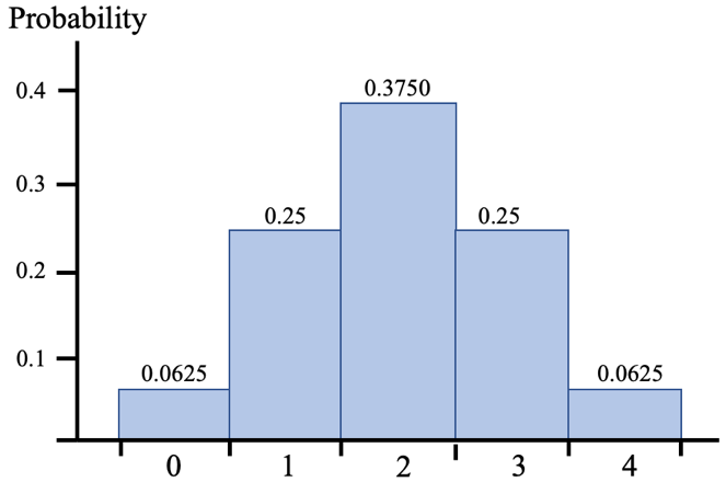
Figure 6.4: Creating a probability histogram for the number of tails when flipping a coin 4 times.

The discrete probability distribution appears to be bell-shaped. The mean appears to be about 2, and most of the time the number of tails is between 1 and 3, inclusive.

Calculating the Mean and Standard Deviation for Discrete Random Variables

A discrete random variable can be described the way we described data in chapters 2 and 3. Specifically, we will describe a probability distribution by addressing the following three characteristics:

•Center- based on the probability distribution, what is the most typical or expected outcome?

•Variation- how much will the outcomes in the probability distribution vary?

•Shape of the distribution- is the probability histogram skewed or bell-shaped?

In the last example we were able to describe the shape by noting that the probability histogram looks reasonably bell-shaped. It appears that 2 is right in the middle, so that is a good guess for the mean. And it doesn’t appear to vary a lot, with bulk of the probability between 1 and 3 inclusive. But can we apply the formulas from chapter 3 to find the mean and standard deviation of a discrete random variable? The answer is... yes!

We won’t derive the formulas but will show how they can be used.

Solution:To find the mean, we can use the formula directly. That will give us the following:

$$\begin{array}{cc}{\mu }_X& =\sum X\cdot P\left(X\right)\\ & =0\times 0.0625+1\times 0.2500+2\times 0.3750+3\times 0.2500+4\times 0.0625\\ & =0+0.25+0.75+0.75+0.25\\ & =2\end{array}$$

So, the mean is 2, which is what looks to be the middle of the probability histogram from figure 6.4. Figure 6.5 shows the probability histogram with the mean ${\mu }_X=2$ added. Notice that the mean is right in the middle, as expected.

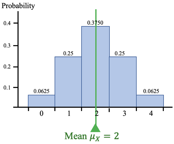
Figure 6.5: Probability histogram for the number of tails with the mean.

To find both the mean and standard deviation by hand, it can sometimes be helpful to organize the probability distribution into a table of columns. For the mean, add a column to the right of the probability column and call it $X\cdot P(X)$. Then, multiply each of the X values by its associated probability and write the result in the third column. The sum of that column is the mean. See figure 6.6.

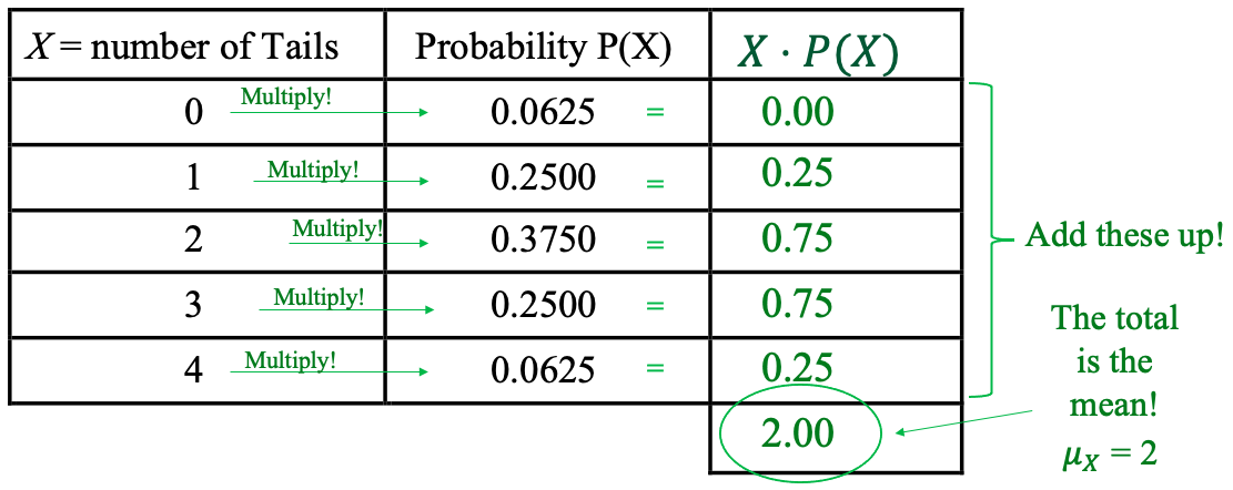
Figure 6.6: Using a table to calculate the mean.

To find the standard deviation, we will add two more columns to the table in figure 6.6. The formula for standard deviation for a discrete random variable is ${\sigma }_X=\sqrt{\sum X^2\cdot P\left(X\right)-{\left({\mu }_X\right)}^2}$. We have already calculated the mean ${\mu }_X$. Next, we need to know the value for $\sum X^2\cdot P\left(X\right)$. First, we will compute $X^2$, then multiply by $P\left(X\right)$, and last find the sum (shown in purple).

Finally, plugging these values into the formula, we arrive at

$$\begin{array}{cc}{\sigma }_X& =\sqrt{\sum X^2\cdot P\left(X\right)-{\left({\mu }_X\right)}^2}=\sqrt{(5)-{\left(2\right)}^2}=\sqrt{5-4}=\sqrt{1}=1\end{array}$$

So, the mean of this discrete random variable is 2, and the standard deviation is 1. That tells us to expect to get two tails, on average, each time we flip a coin 4 times. The standard deviation equal to 1 tells us to expect to be within 1 tail of the mean, most of the time. Taken together, the mean and standard deviation tell us we should see between 1 and 3 tails, most of the time. As we have seen from the probability distribution, you should get between 1 and 3 tails, inclusive, 87.5% of the time that you flip a coin 4 times.

Solution:There are 6 possible outcomes when you roll a six-side die, and each one is equally likely. So, the probability for any of the results is 1/6. The probability distribution is shown in Table 4.

The probability histogram looks like a rectangle, since all the probabilities are the same. This is an example of what is called a uniform distribution, so named because the probabilities are “uniformly the same for each outcome”. The probability histogram is shown in figure 6.7.

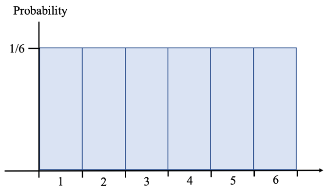
Figure 6.7: Probability histogram for rolling a six-sided die.

To find the mean and standard deviation, we add to Table 4, as we did in example 6.

Using the formulas for the mean and standard deviation of a discrete random variable, we find that the mean number showing on a six sided die is

$$\begin{array}{cc}& \mu =\sum X\cdot P\left(X\right)=3.5\end{array}$$

and the standard deviation of the number showing on a six-sided die is

$$\begin{array}{cc}{\sigma }_X& =\sqrt{\sum X^2\cdot P\left(X\right)-{\left({\mu }_X\right)}^2}=\sqrt{\left(\frac{91}{6}\right)-{\left(3.5\right)}^2}\\ & \approx \sqrt{15.16666667-12.25}\\ & =\sqrt{2.916666667}\\ & \approx 1.708\end{array}$$

The probability distribution for the roll of a six-sided die has the following characteristics.

•Center- The mean, or average roll is 3.5.

•Variation- The standard deviation is approximately 1.708.

•Shape- The probability distribution is uniform, not bell-shaped.

Now, how can technology help us with this process? Can we use STATBELT Utility- the Statistical Basics Exploratory Learning Tool (opens in a new tab) to do any of this work? Luckily, the answer is yes!

We will now revisit examples 3 and 4 using STATBELT.

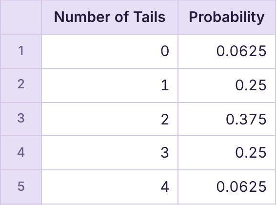
Solution:First, open STATBELT Utility and type 0, 1, 2, 3, and 4 in the first column of the spreadsheet, and the probabilities in the next column. Name the columns “Number of Tails” and “Probability”.

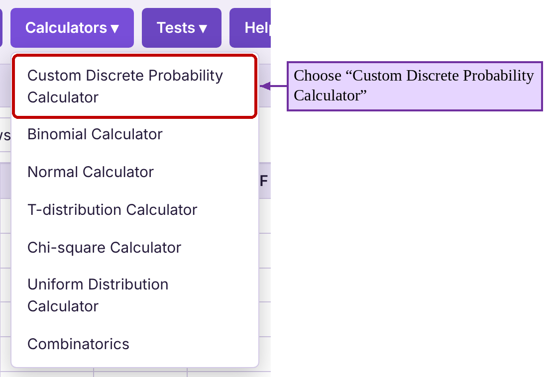
Next, select Calculators → Custom Discrete Probability Calculator.

Choose “Number of Tails” for “X values in” and “Probability” for “Probabilities in.”

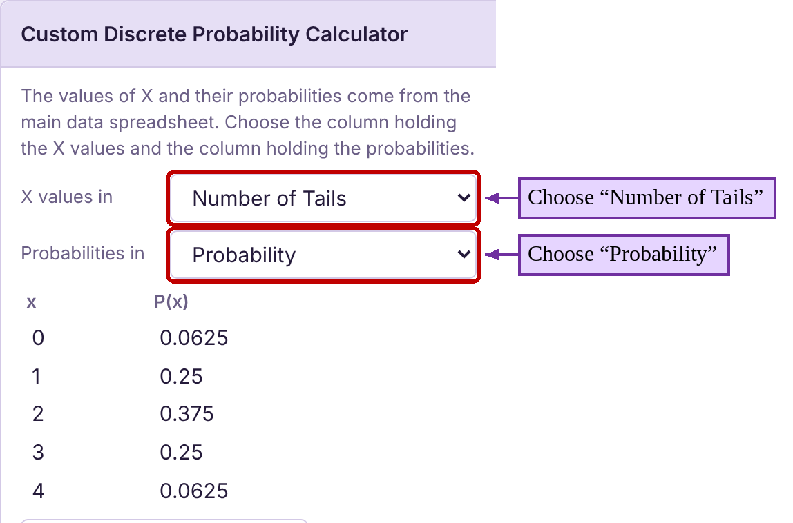
The custom calculator appears as soon as both columns are chosen. There is no button to click.

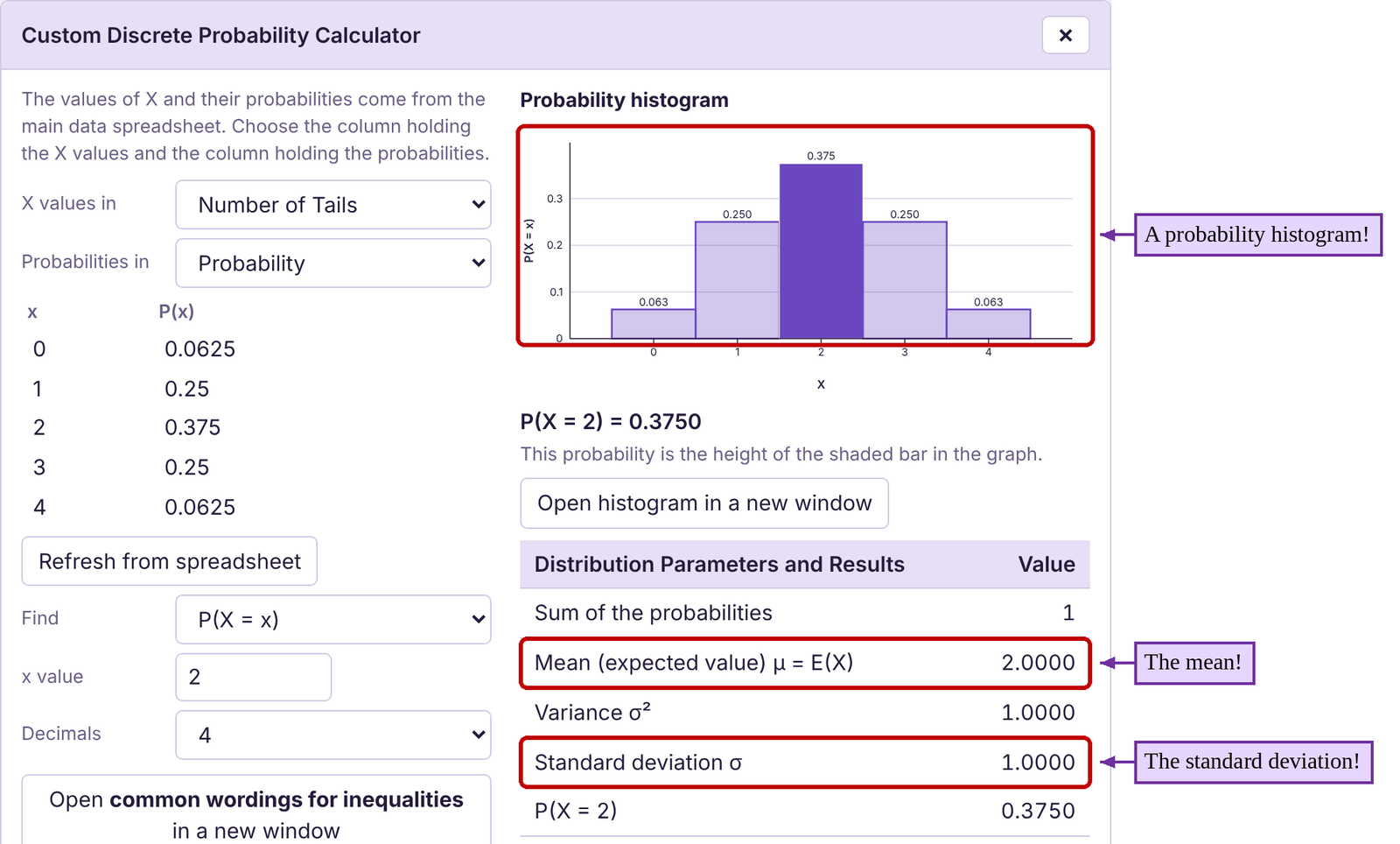
Note that the mean and standard deviation have been calculated for you. The mean is shown to be 2, and the standard deviation has been calculated to be 1. There is also a probability histogram, with one bar for each value of X. The height of each bar is the probability of that value. To use the calculator to find the probabilities of different events, we can change the inequality under “Find” and the number or numbers we compare to X. To see a larger histogram, click “Open histogram in a new window.”

a)To find $P\left(X=2\right)$, set the inequality to $"="$ by choosing P(X = x) under “Find,” and type 2 for the x value. We could have read this from the table, but it is good to see that the calculator tool agrees. Note that the bar at 2 is shaded dark purple. When using the tool, the shaded bars correspond to the probability you select.

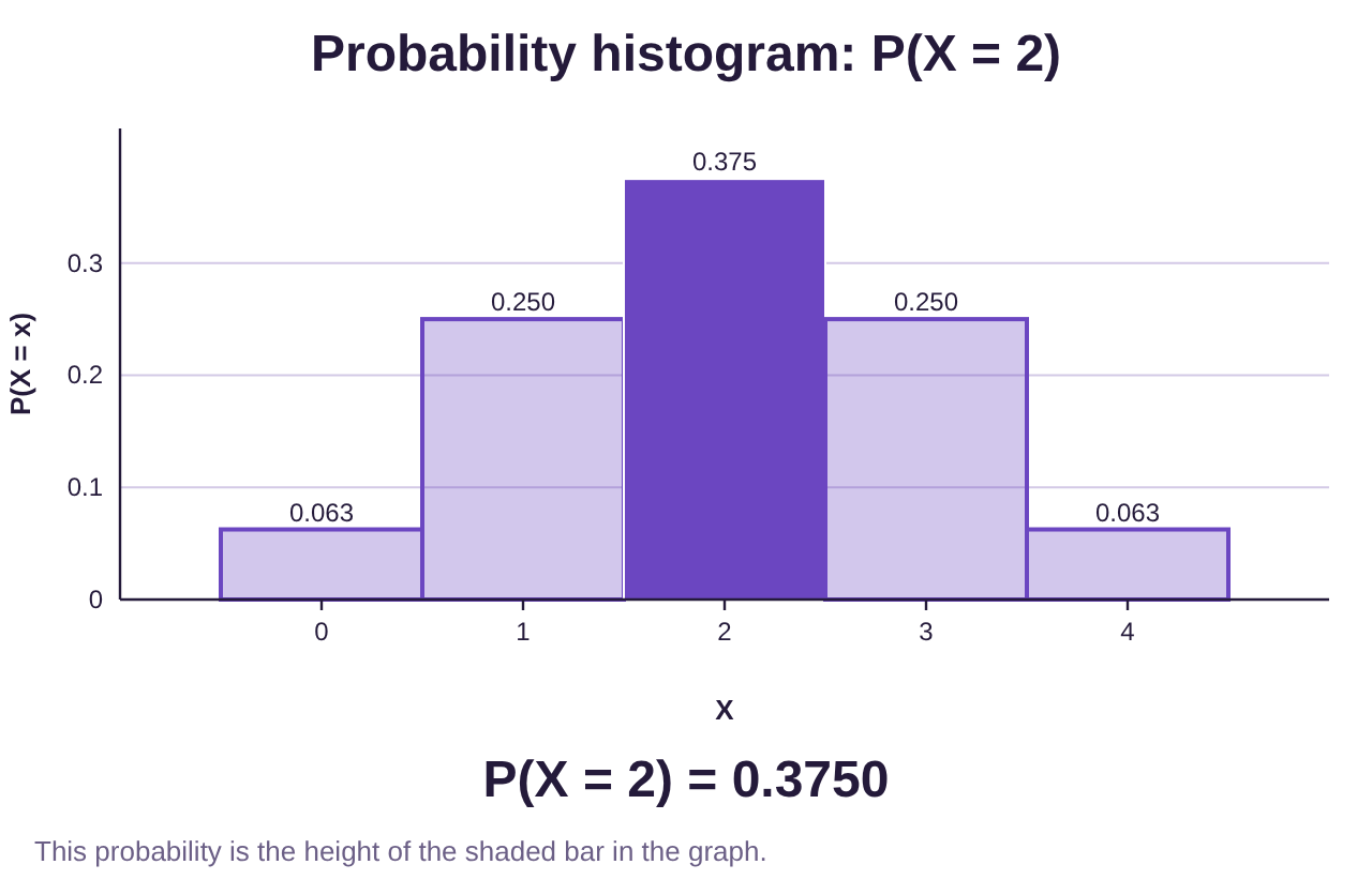
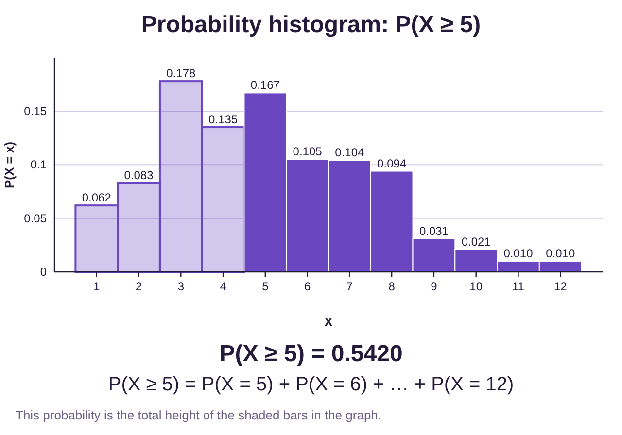
b)To find the probability that X is greater than or equal to 2, set the inequality to $"\ge "$ by choosing P(X ≥ x), and leave the x value at 2. Here the bars for 2, 3, and 4 are shaded, and the probability is 0.6875, agreeing with our previous work.

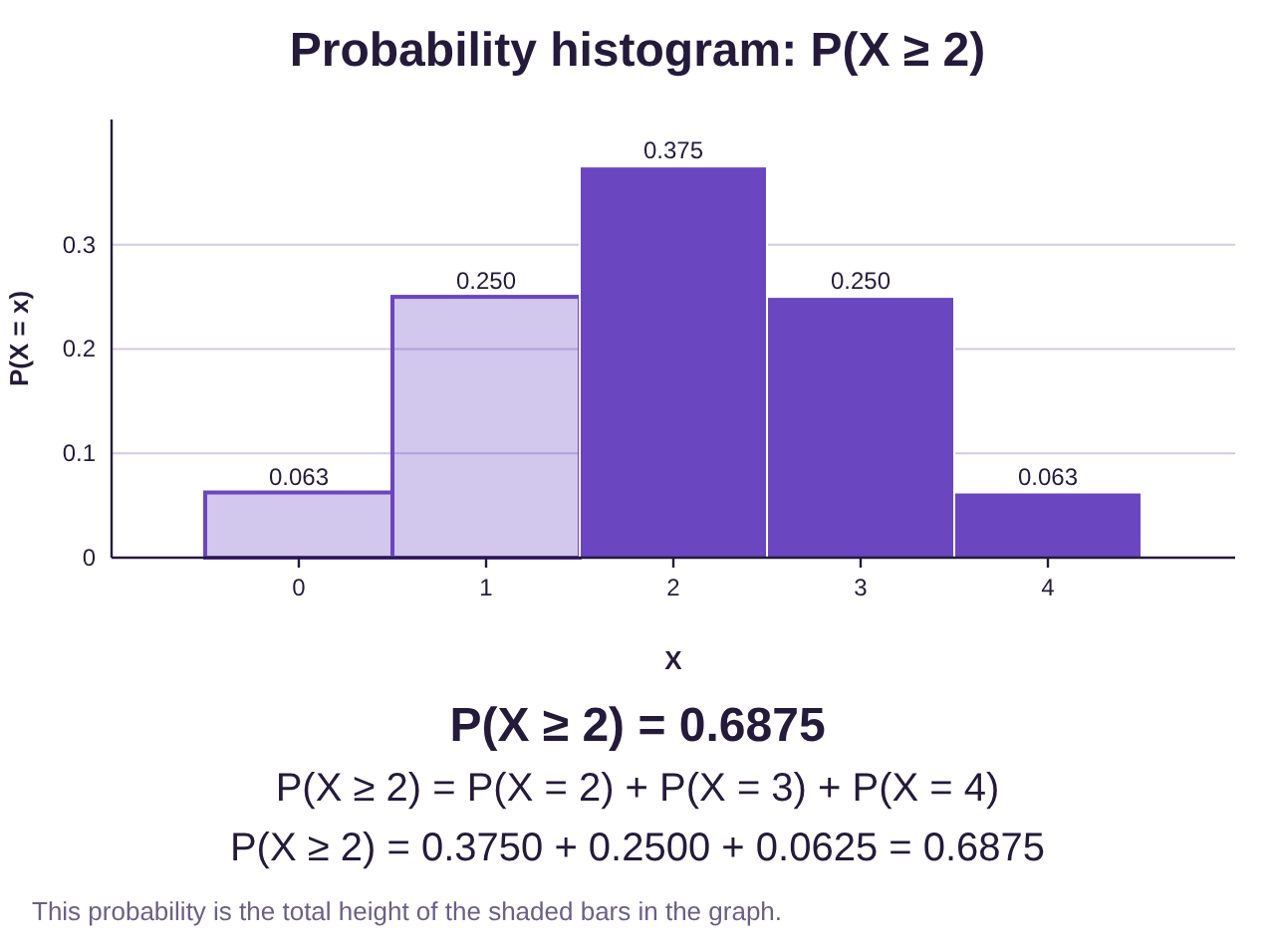
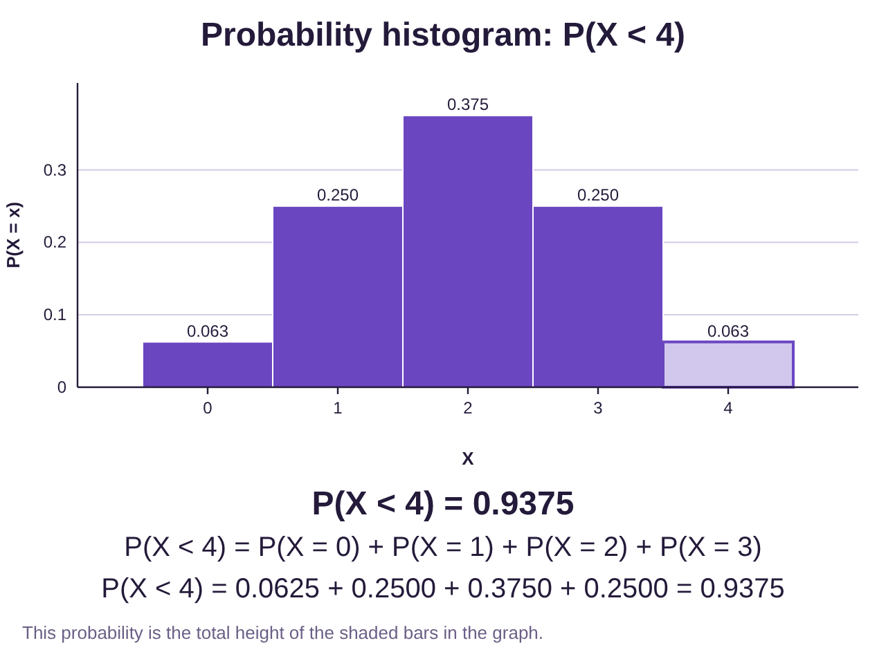
c)To find the probability of fewer than 4 tails, set the inequality to $"<"$ by choosing P(X < x), and change the x value to 4. The bars that are “fewer than 4” are shaded, and the probability is 0.9375.

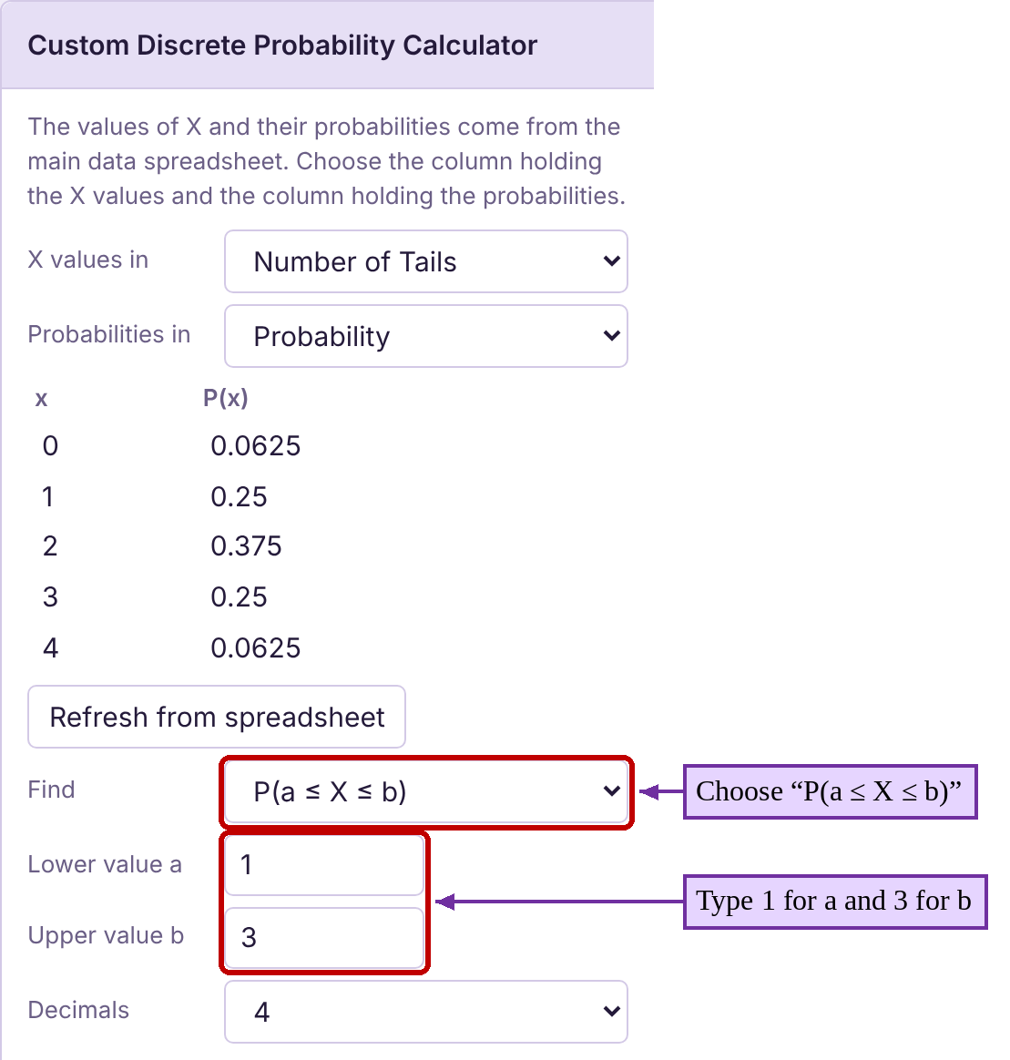
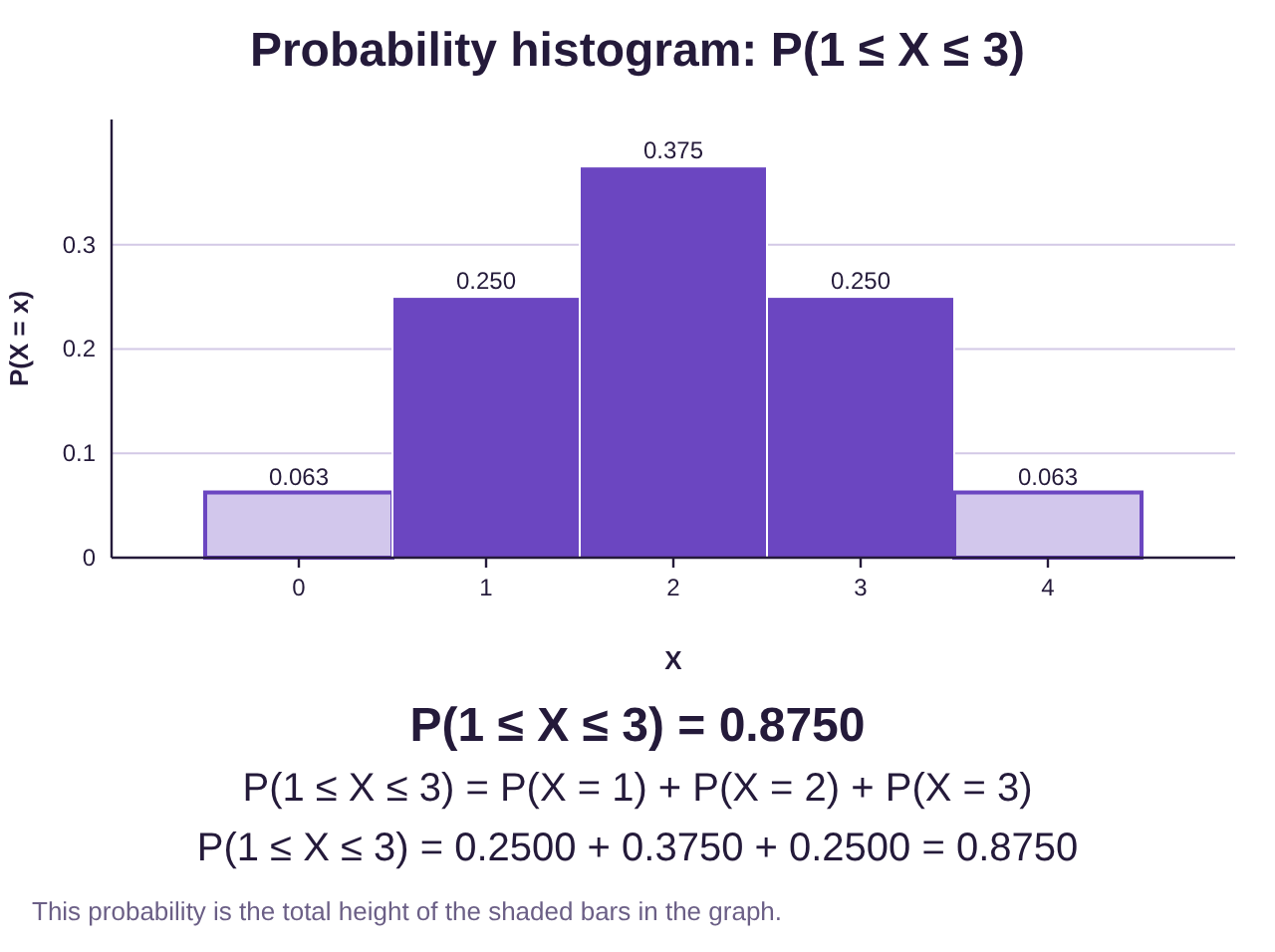
d)To find the probability that the number of tails is between 1 and 3, inclusive, we use the “between” setting. We want to find $P\left(1\le X\le 3\right)$, so choose “P(a ≤ X ≤ b)” under “Find.” Notice that the inequalities for between are always $"\le X\le "$. Type 1 for the lower value a and 3 for the upper value b. The result is $P\left(1\le X\le 3\right)=0.875$.

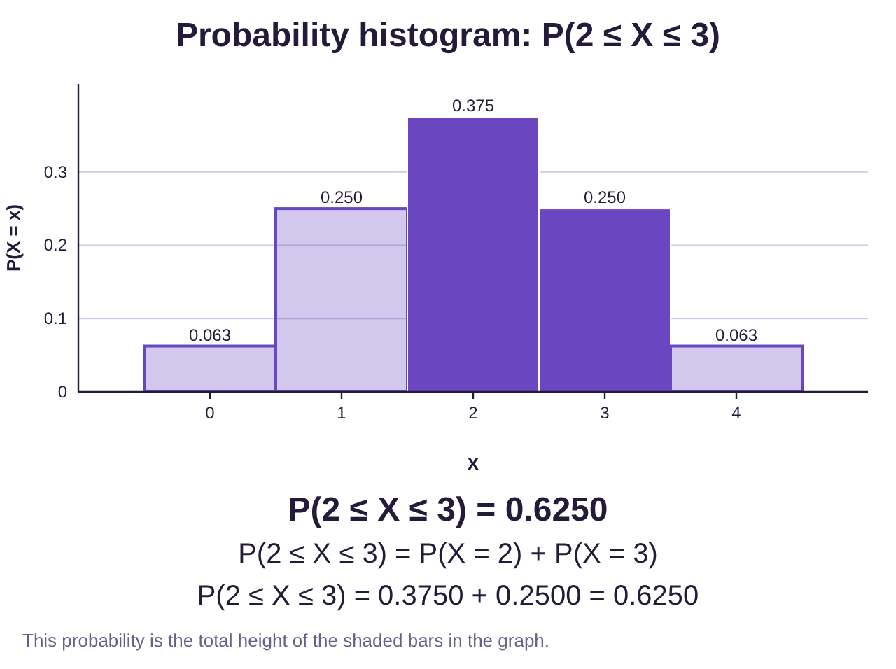
e)To find $P\left(1<X<4\right),$ we can use the “between” setting, P(a ≤ X ≤ b), but there is no option to change it to “ < X < ”. So, in this case, we need to interpret $P\left(1<X<4\right)$ using the less than or equal to inequalities, $"\le X\le ".$ The numbers that are between 1 and 4 are X = 2 and X = 3. Type 2 for a and 3 for b. The result is $P\left(1<X<4\right)=P\left(2\le X\le 3\right)=0.625$.

Solution:First, open STATBELT Utility and type 0, 1, 2, 3, 4, and 5 in the first column of the spreadsheet, and the probabilities in the next column. Name the columns “Number of Green Lights” and “Probability”.

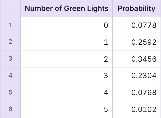
Select Calculators → Custom Discrete Probability Calculator, and choose “Number of Green Lights” for “X values in” and “Probability” for “Probabilities in.”

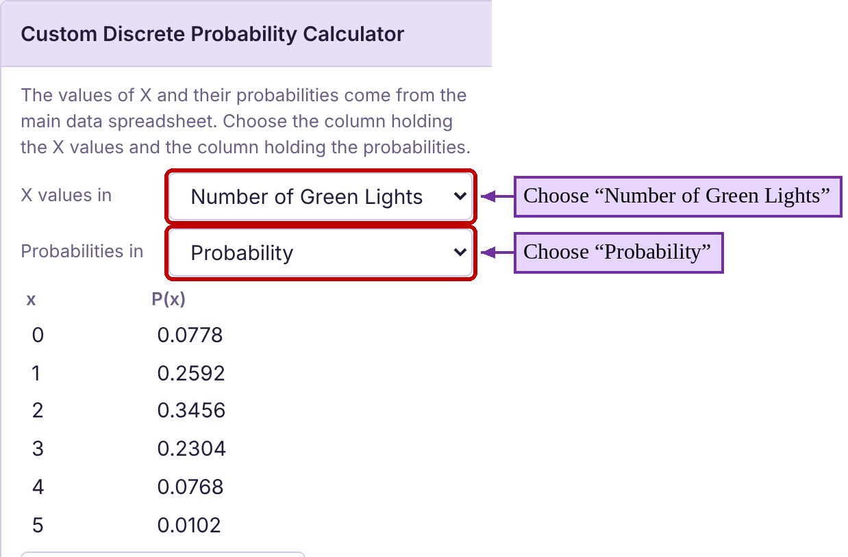
The custom calculator is shown in figure 6.8.

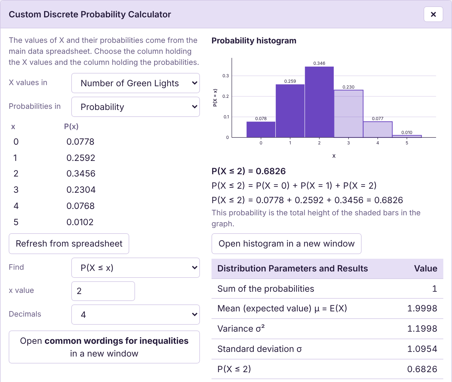
Figure 6.8: The custom calculator in STATBELT Utility.

a)To describe the distribution, we identify the center, variation, and shape.

•Center- STATBELT has calculated the mean to be ${\mu }_X=1.9998\approx 2$. The student should expect to see 2 green lights, on average, while driving to school.

•Variation- The standard deviation is ${\sigma }_X=1.095\approx 1.1$. That means that the student should expect to see 2 green lights, plus or minus 1.1, most of the time. Effectively, this means she will most often see between 1 and 3 green lights on a trip to school.

•Shape of the distribution- The probability histogram appears close to bell-shaped, but with a slight skew to the right.

b)Under “Find,” choose P(X ≥ x) (the inequality “$\ge$”), and type 3 for the x value. The probability she will see at least three green lights is $P\left(X\ge 3\right)=0.3174$.

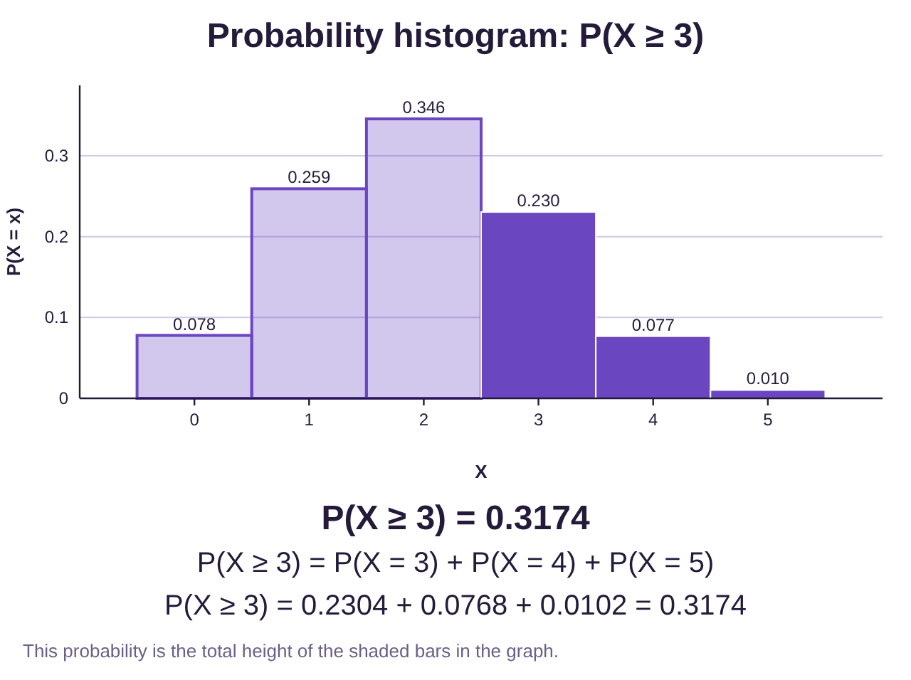
c)Choose P(a ≤ X ≤ b) under “Find,” and type the endpoints 1 and 4 for a and b. The probability she will see between 1 and 4 lights, inclusive, is $P\left(1\le X\le 4\right)=0.912$.

Solution:a)To describe how many 3-point shots you expect him to make, we will compute the mean and standard deviation of DRV X = Number of 3-point shots made. You can either type the data into two columns of the STATBELT spreadsheet or open the Table 5 data (opens in a new tab) in STATBELT (download CSV). Then select Calculators → Custom Discrete Probability Calculator, and choose “3-pointers” for “X values in” and “Probability” for “Probabilities in.” The custom calculator is shown in figure 6.9.

Photo by Markus Spiske (opens in a new tab) on Unsplash (opens in a new tab)

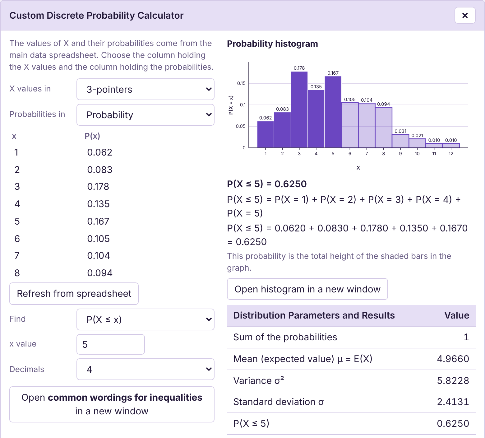
Figure 6.9: Custom calculator for Steph Curry 3-point shots.

The mean number of 3-point shots he makes is ${\mu }_X=4.966\approx 5$. So, he makes 5 three-point shots per game, on average. The standard deviation is ${\sigma }_X=2.4131\approx 2.4$. This can be interpreted as “most of the time, Steph Curry will make 5 plus or minus 2.4 three-point shots in a game.” Thus, most of the time he will make between 3 and 7 shots, inclusive. If you attend a game in which he plays, he will likely make between 3 and 7 three-point shots.

b)The likelihood he makes at least 5 shots is $P\left(X\ge 5\right)\approx 0.542$.

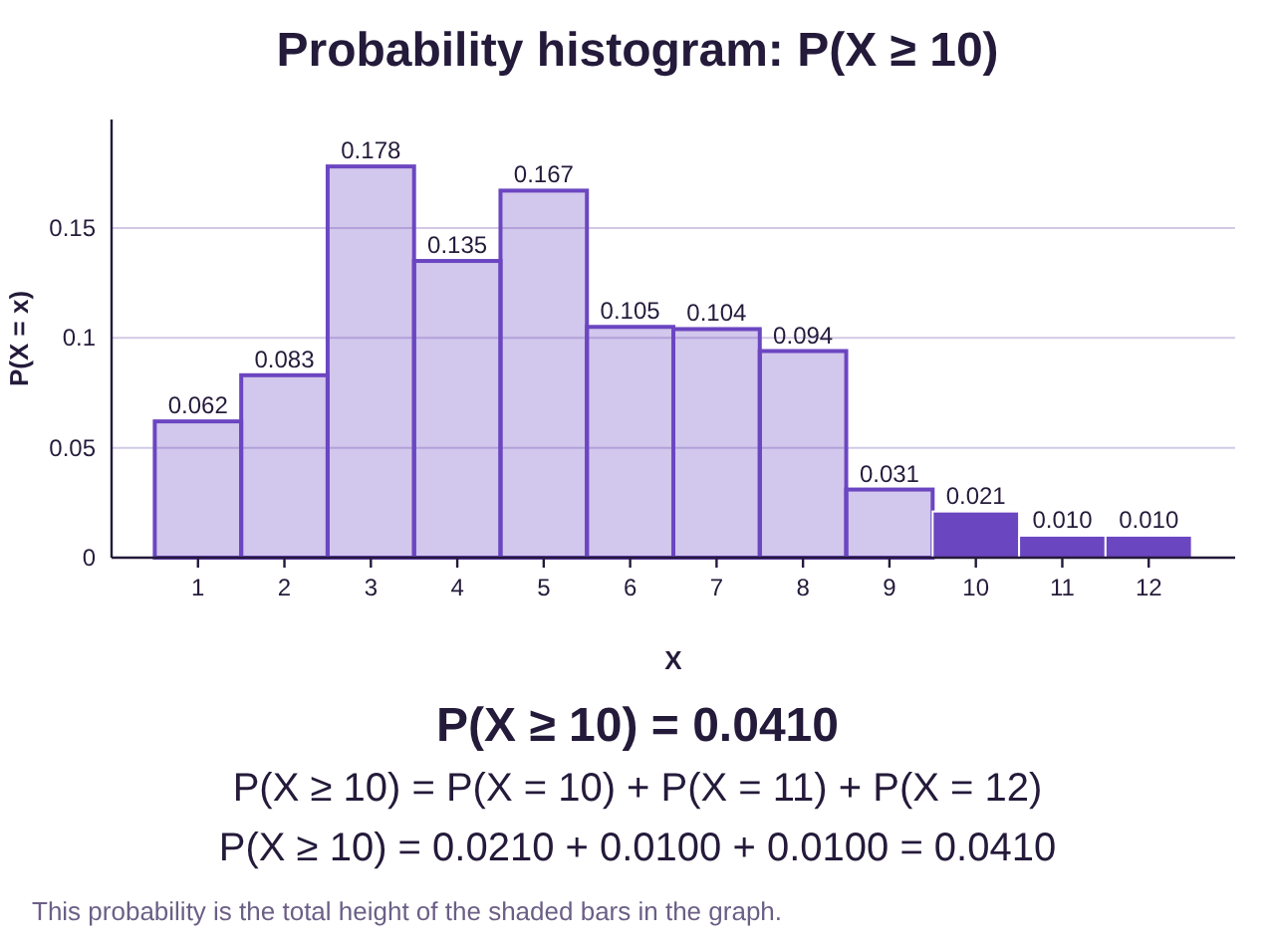
c)The likelihood he makes at least 10 shots is $P\left(X\ge 10\right)\approx 0.041$. Since the probability is less than 0.05, there is less than a 5% chance he will make 10 or more three point shots. If he did, it would be unusual.

Expected Value

The expected value of a discrete random variable is another name for the mean. Basically, what you “expect” to happen is what happens “on average”, which is the mean. In gambling and insurance, if we call X the amount you can win or lose per attempt, the expected value is the amount you expect to win or lose for each attempt, on average. To calculate expected value, make a list of each possible amount that could be won or lost, and the probability of each event. The mean is the expected value!

Solution:First, there are only two possible outcomes to this game. You will either (1) roll at least one six and win $5, or (2) roll no six and lose $5. The probability that you win is $P\left(\text{Win }\$5\right)=0.518$, so using the complement, the probability that you lose is $P\left(\text{Lose }\$5\right)=1-0.518=0.482$. We can organize this information in a table, shown in Table 6.

Notice that we used a negative for the amount that you lose. We interpret winning as positive and losing as negative.

a)To find the expected value, we can multiply each X by its probability, and find the sum.

Table 6: Outcomes of 4-dice Rolling Game
Outcome	X = Amount won or lost	Probability	$$\begin{array}{cc}& X\cdot P(X)\end{array}$$
Roll a six	5	0.518	2.59
Don't roll a six	-5	0.482	-2.41
			0.18

The mean is 0.18, which is interpreted in the following way. You should expect to win an average of $0.18 per game you play. If you prefer, you can copy the table into STATBELT and use the Custom Discrete Probability Calculator. But, with only two outcomes to multiply, it did not take much work to find the expected value by hand.

b)For 100 bets, multiply the expected value per game by the number of bets: $\$0.18\times 100=\$18.$ You should expect to make about $18. Certainly not a lot for that many bets, but since the probability of winning and losing are very close, you should expect to win only slightly more often than you lose.

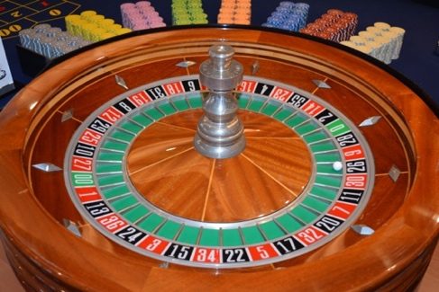
Photo by Derek Lynn (opens in a new tab) on Unsplash (opens in a new tab)

Solution:a)The “straight up” bet has a probability of winning of 1/38, and a probability of losing of 37/38. So, the expected value can be calculated by finding the mean of the discrete probability distribution in Table 7.

Since the expected value is -0.526, the player should expect to lose about $0.53 per “straight up” bet placed.

b)The “Red” bet has a probability of winning of 18/38, and a probability of losing of 20/38. So, the expected value can be calculated by finding the mean of the discrete probability distribution in Table 8.

Since the expected value is -0.526, the player should expect to lose about $0.53 per “Red” bet placed.

c)The “First dozen” bet has a probability of winning of 12/38, and a probability of losing of 26/38. So, the expected value can be calculated by finding the mean of the discrete probability distribution in Table 9.

Once again, the expected value is -0.526, so the player should expect to lose about $0.53 per “First dozen” bet placed.

You may have noticed that the expected value is the same for all three bets. That means that regardless of the type of bet placed, the casino expects to make about $0.53 per bet. The player should expect to lose the same amount. If there are 1000 bets placed on a roulette table in an evening, those bets add up to about $1000\times \$0.53=\$530$ of profit for the casino. The expected value when not making a bet is zero, so your best bet is to not make a bet in a casino!

Tip!

Casinos are not the only example of negative expected values. Any insurance policy is a gamble. If you need the insurance over the duration of the policy, you win the bet. If you don’t need the insurance, you lose the bet and the cost of the policy. Insurance policies generally have negative expected values, just like games in a casino. But some insurance, such as car insurance, is required by law. Other types of insurance, like home-owners insurance, is required to borrow money for a home purchase. Still others, like life or disability insurance, provide financial resources in devastating situations when you may be unable to provide for your family. Just because insurance has a negative expected value does not make it a poor decision to purchase it.

Extended warranties are another example. When you purchase an extended warranty for a car or electronic device, you are gambling that you will need it. If you don’t use the warranty, you have lost the bet (and lost the cost of the extended warranty). If you need to use the warranty, you have won the bet and win the repair or replacement cost of the item. But you should be aware that the prices of those extended warranties are set so that the expected value is negative for you, meaning that the company will expect to make money for each extended warranty sold. For that reason, extended warranties are widely considered by consumer advocates to be a poor investment. That said, there are plenty of examples of someone who benefitted from one. If you are particularly hard on watches, you might want to buy the extended warranty when you purchase a watch. But if not, it might be best to keep your money. The cost of repair is often only slightly higher than the cost of the warranty.