Section 7.2: The Normal Distribution

The normal distribution can be described using the same three characteristics that we have seen.

•Center- Since it is bell-shaped, we use the mean to describe the center.

•Variation- Since it is bell-shaped, we use standard deviation to describe the dispersion.

•Shape of the distribution- It is normal, so we know it is bell-shaped.

Thus, the normal distribution is completely determined by the mean and standard deviation (we get that it is bell-shaped since we know it is normal). We use technology to find probability as the area under the normal probability density function. When we do, we will need to specify 1) the mean, 2) the standard deviation, and 3) that the probability density function follows a normal distribution.

The Standard Normal Distribution

First, it is important to know the history behind the standard normal, or Z-distribution.

The Standard Normal Distribution is the bell-shaped distribution that was once used to compute probabilities for any normal curve. The process required users to convert X-values to standardized scores (remember z-scores?) using the mean and standard deviation, then use tables of values to look up probabilities. Carl Friedrich Gauss was the first person to discover and use the normal distribution, hence it is sometimes called the Gaussian distribution. At the time of its discovery, there was no technology to use, so scientists spent hours, days, and weeks creating tables of values for areas under the standard normal curve. Although it is possible to compute tables for every combination of mean and standard deviation, it made better sense to adopt a standard, then have all others convert to the standard when computing probability. Because it was the simplest to compute, the standard normal distribution has mean $\mu =0$ and standard deviation $\sigma =1.$ This is what tables use as the “standard” and is the default if you are using a probability calculator (like Desmos, an app, or STATBELT). When we refer to the standard normal variable, we use Z. When we refer to any other normal distribution, we use X.

Solution:Open STATBELT Utility and select Calculators → Normal Calculator. The mean is already 0 and the standard deviation is already 1.

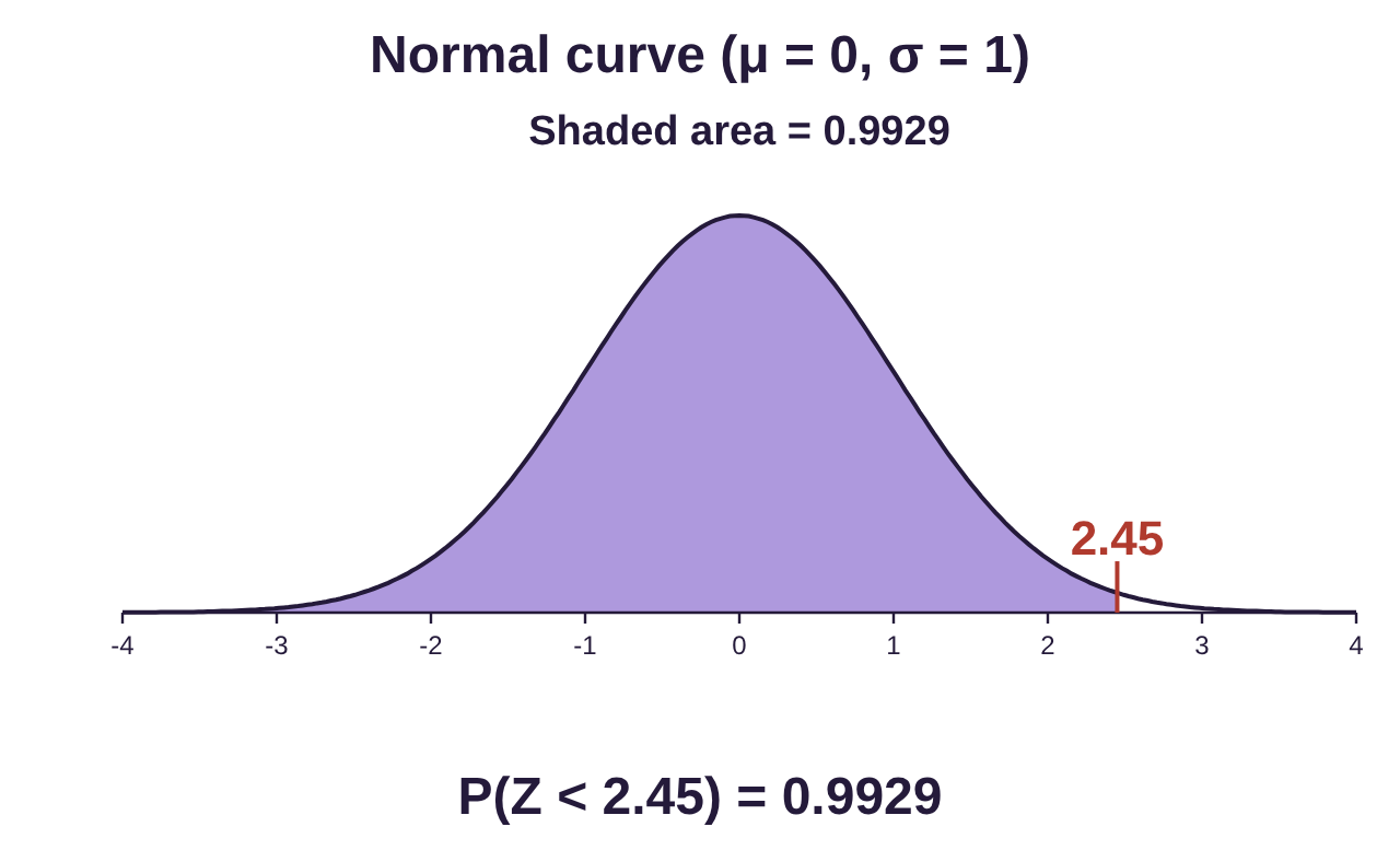
a)To compute $P\left(Z<2.45\right),$ choose “P(Z < z)” and type 2.45 for the z value. The result is $P\left(Z<2.45\right)\approx 0.9929.$

The calculator also gives you a picture of the distribution. The shaded area between the curve and the axis represents the probability of getting a value of the random variable in that interval. Notice that the solution to $P\left(Z<2.45\right)=P(Z\le 2.45)$ This is always true of continuous random variables.

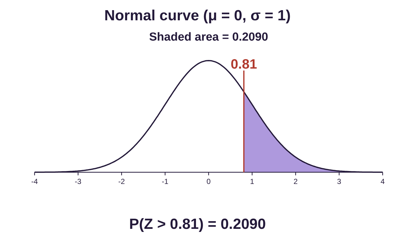
b)To compute $P\left(Z>0.81\right),$ choose “P(Z > z)”

and type 0.81 for the z value. The result is $P\left(Z>0.81\right)\approx 0.2090,$ rounded to 4 decimal places. Again, there is no difference using “$\ge$” instead of “>” because we are working with a continuous random variable.

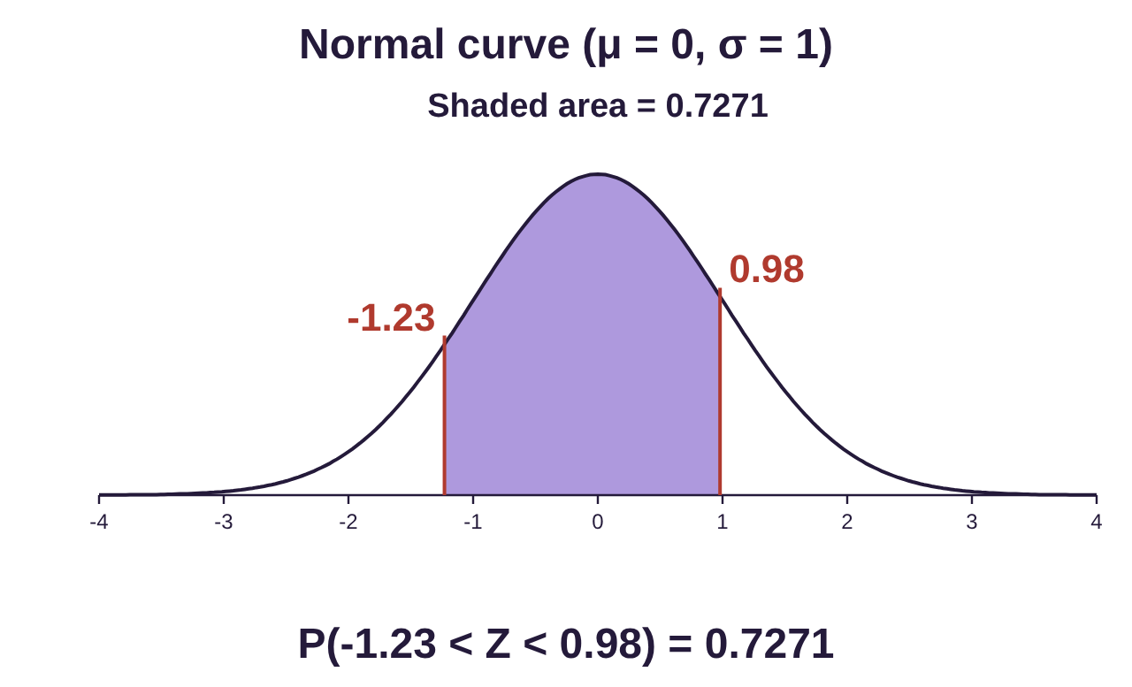
c)To calculate $P(-1.23<Z<0.98)$, choose “P(z₁ < Z < z₂)” under “Find a probability.” Type -1.23 for the lower value and 0.98 for the upper value. The result is $P\left(-1.23<Z<0.98\right)\approx$ 0.7271, rounded to 4 decimal places. You might notice that the calculator writes “less than” (<) rather than “less than or equal to” (≤). When the variable is continuous, the probability of being “equal” to any number is zero, so these two options give the same area, and therefore the same probability.

Solution:Open STATBELT Utility and select Calculators → Normal Calculator. The mean is already 0 and the standard deviation is already 1.

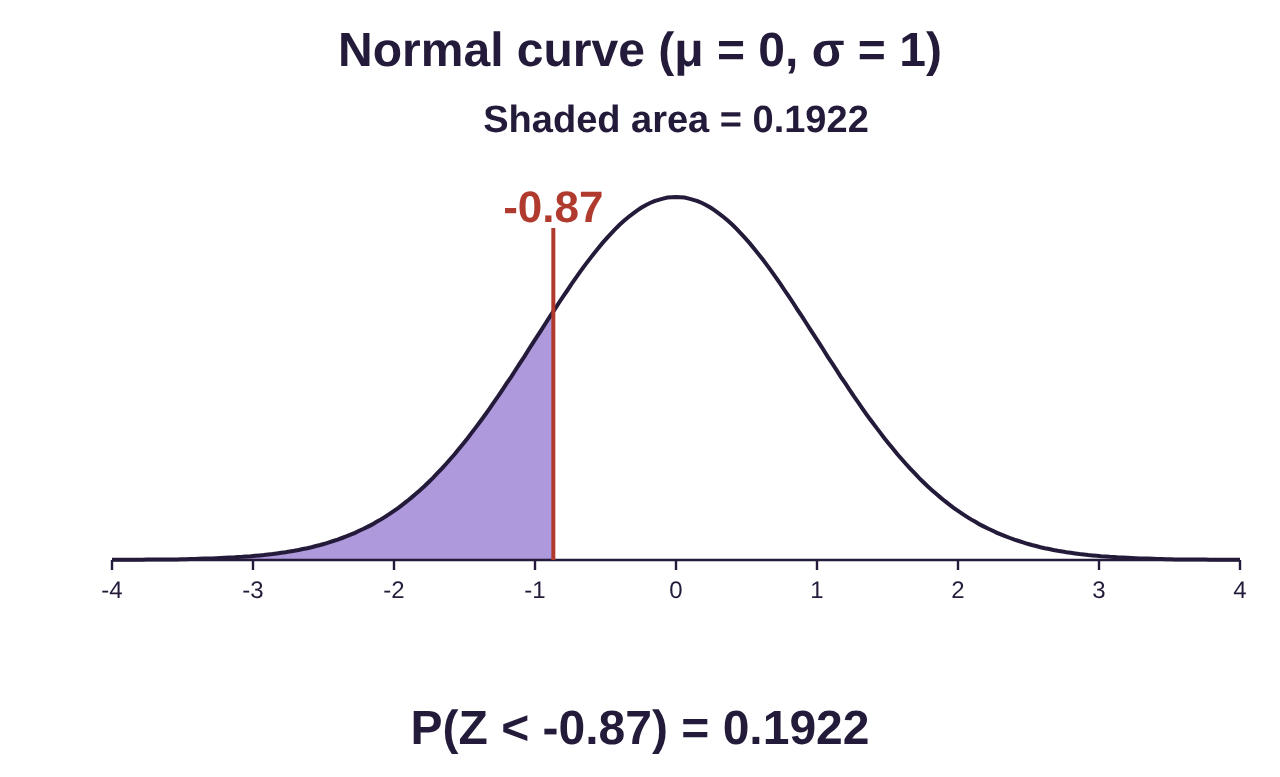
a)The area to the left of -0.87 is equal to the probability $P\left(Z<-0.87\right).$ Choose “P(Z < z)” and type

-0.87 for the z value. The result is $P\left(Z<-0.87\right)\approx 0.1922$. There is about a 19.2% chance that a standard normal variable is less than

-0.87.

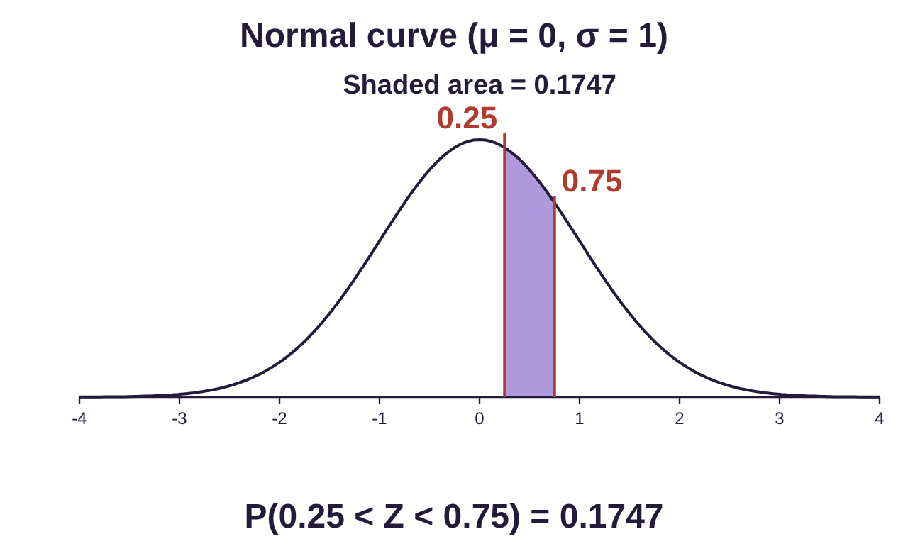
b)The area between 0.25 and 0.75 is the same as the probability $P\left(0.25<Z<0.75\right)$. Choose “P(z₁ < Z < z₂)” and type 0.25 for the lower value and 0.75 for the upper value. The result is $P\left(0.25<Z<0.75\right)\approx$ 0.1747. Approximately 17.5% of standard normal values are between 0.25 and 0.75.

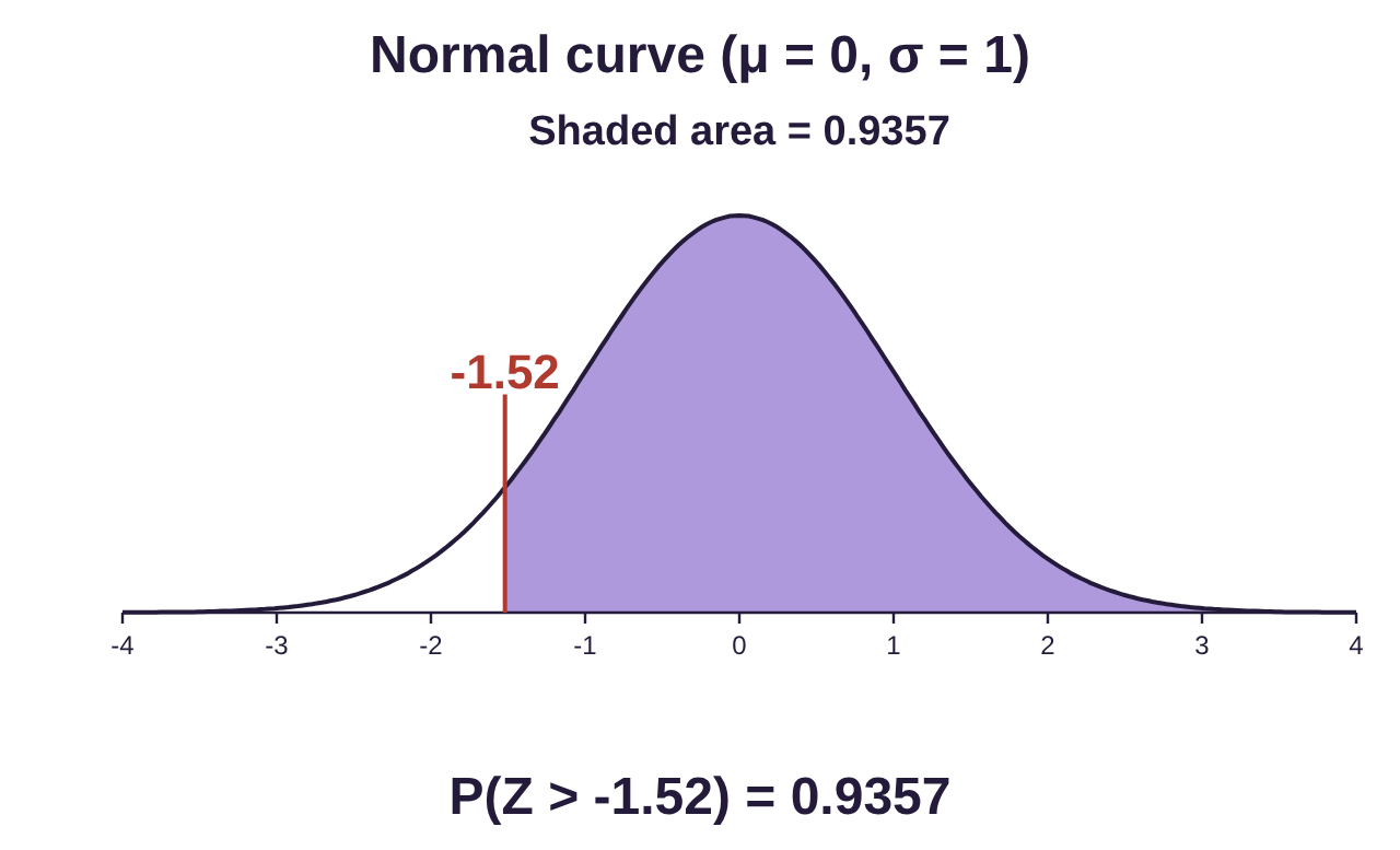
c)The area to the right of -1.52 is the same as the probability $P\left(Z>-1.52\right)$. Choose “P(Z > z)” and type

-1.52 for the z value. The result is $P\left(Z>-1.52\right)\approx$ 0.9357. A standard normal variable will be larger than -1.52 approximately 93.6% of the time.

The Non-Standard Normal Distribution

Historically, when probability was computed for non-standard normal variables X, they had to first be converted to the standard normal using z-scores. You may recall using z-scores in chapter 3.

If we apply the z-score formula to a normal distribution with mean $\mu$ and standard deviation, $\sigma ,$ we convert the non-standard normal into the standard normal. That is, the mean is converted to 0 and the standard deviation is converted to 1. Once this was necessary to compute probability. After converting to the standard normal, statisticians would use tables to make very complicated estimates for the probability. The next example is presented to show how the areas of the non-standard normal and the standard normal are equivalent in this process. Fortunately, we have technology that we will use to compute these probabilities.

Solution:a)Substituting values X = 66, $\mu =72$ and $\sigma =8,$ into the Z-score formula, we get

$$\begin{array}{cc}Z& =\frac{66-72}{8}=-\frac{6}{8}=-0.75\end{array}$$

The interpretation of the Z-score from chapter 3 is that the value X = 66 is 0.75 standard deviations below the mean. (Recall it is below because of the negative sign.)

b)If Z = 1.6, then we can compute the raw score for $X$ as

$$\begin{array}{cc}X& =\mu +Z\cdot \sigma \end{array}$$

$$\begin{array}{cc}& =72+1.6\times 8\\ & =72+12.8\\ & =84.8\end{array}$$

So, the raw score X = 84.8 is 1.6 standard deviations above the mean.

c)To see how we transform a non-standard normal distribution to a standard normal, we start with $X<66.$ Using algebra, we can subtract the mean from both sides, and divide by both sides by the standard deviation.

$$\begin{array}{cc}& X<66\end{array}$$

$$\begin{array}{cc}& X-72<66-72\end{array}$$

$$\begin{array}{cc}& \frac{X-72}{8}<\frac{66-72}{8}\end{array}$$

$$\begin{array}{cc}& Z<\frac{-6}{8}\end{array}$$

$$\begin{array}{cc}& Z<-0.75\end{array}$$

So, the inequalities “$X<66$” and “$Z<-0.75$” are equivalent via the Z-score transformation. It turns out that the areas under the transformed graphs are also equal, and hence the probabilities are equal.

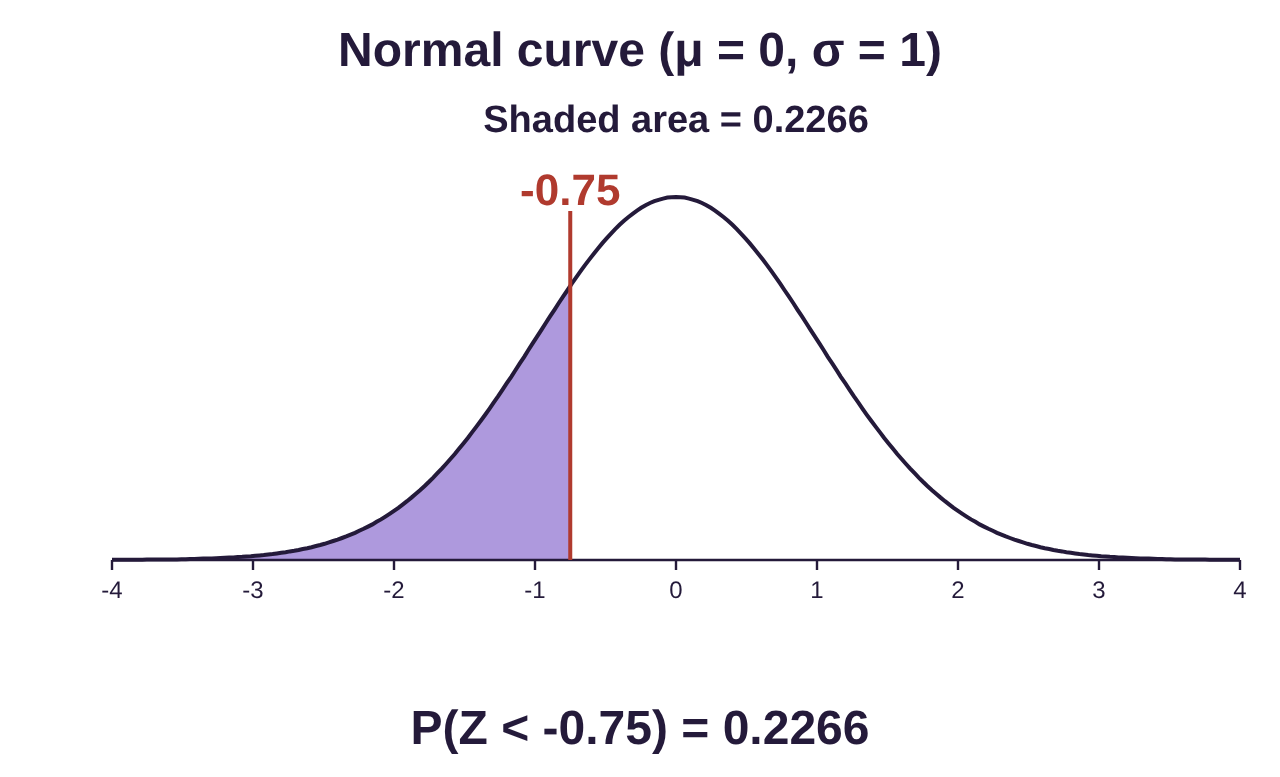
To find the probability $P(Z<-0.75)$, open STATBELT Utility and select Calculators → Normal Calculator. With mean set to 0 and standard deviation set to 1, choose “P(Z < z)” and type -0.75 for the z value.

$P\left(X<66\right)=P(Z<-0.75)$. Using STATBELT, $P\left(Z<-0.75\right)\approx 0.2266$. So, the probability that a randomly selected X is less than 66 is approximately 0.2266.

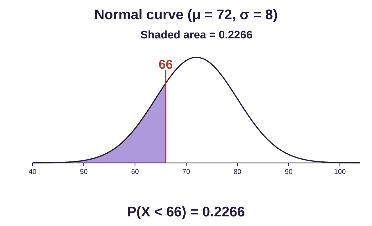
Note that if we had changed the mean and standard deviation in the normal calculator to 72 and 8, respectively, and found $P\left(X<66\right)$, we get $P\left(X<66\right)\approx 0.2266$, the same probability!

The main point of this last example is to show that we don’t need to convert to the standard normal to find probability for a normal distribution! But we do need to use the standard normal in future chapters, so it is important to know what it is.

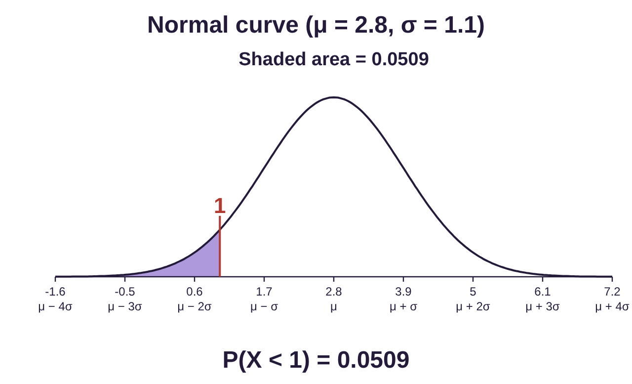
Solution:a)Open STATBELT Utility and select Calculators → Normal Calculator. Type in 2.8 for the mean and 1.1 for the standard deviation. To find the probability that a phone is replaced before it is a year old, we find $P(X<1)$. We don’t need to convert to Z-scores. Just choose “P(X < a)” and type 1 for the value a. If you set “x-axis labels” to “Mean ± standard deviations,” the normal distribution that is presented will match what we created in section 7.1 example 5. The result is $P\left(X<1\right)\approx 0.0509$. There is just over a 5% chance that a cell phone will be replaced before it is one year old. Since this is not less than 0.05, it is not unusual. It is, however, close to unusual!

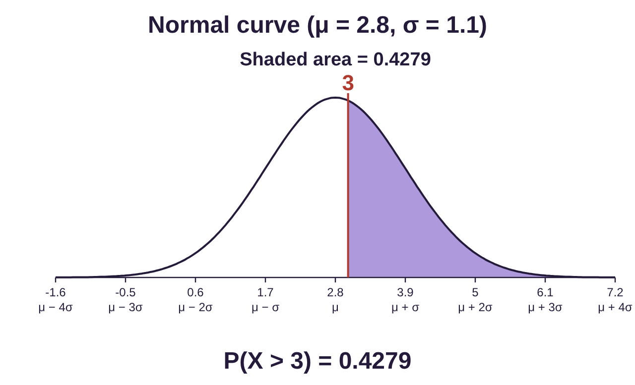
b)To find the probability that a phone lasts at least 3 years, we find $P(X>3)$. Choose “P(X > a)” and type 3 for the value a. We get $P\left(X>3\right)\approx 0.4279$. There is a 42.8% chance that a cell phone will last at least 3 years.

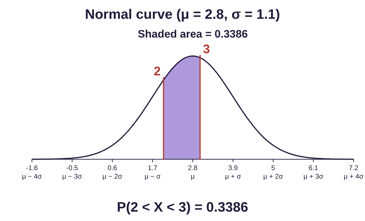
c)To find the probability that a phone lasts between 2 and 3 years, we find $P(2<X<3)$. Choose “P(a < X < b)” and type 2 for the lower value a and 3 for the upper value b. We get $P\left(2<X<3\right)\approx 0.3386$. Approximately 33.9%, or just over one-third of cell phones are replaced between 2 and 3 years.

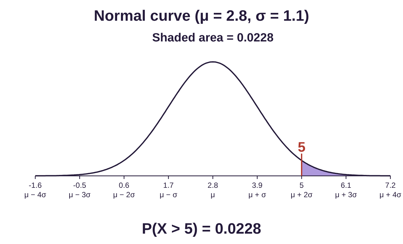
d)To find the probability that a phone lasts longer than 5 years, we find $P(X>5)$. Choose “P(X > a)” and type 5 for the value a. We get $P\left(X>5\right)\approx 0.0228$. Approximately 2.3% of cell phones last longer than 5 years. Since this is less than a 5% chance, it would be unusual to have a cell phone used longer than 5 years.

Tip!

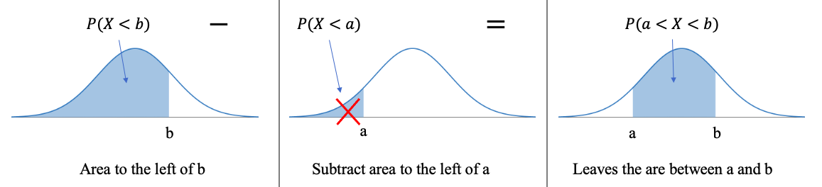
Figure 7.18: How to compute a between probability using two left-tail probabilities.

Solution:Open STATBELT Utility and select Calculators → Normal Calculator. Type in 268 for the mean and 16 for the standard deviation. Set “x-axis labels” to “Mean ± standard deviations” to show the mean and increments of the standard deviation.

a)To find the probability that a pregnancy lasts less than 250 days, we find $P(X<250)$. Choose “P(X < a)” and type 250 for the value a.

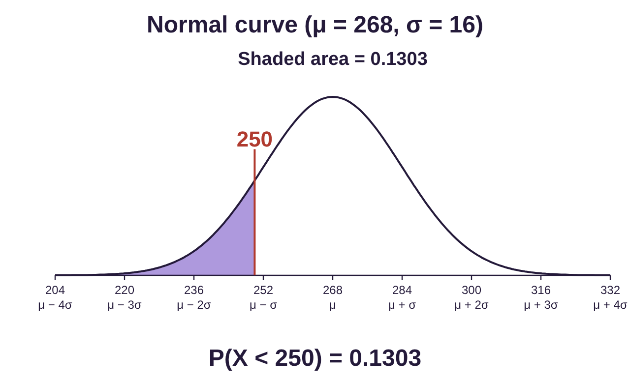
The result is $P\left(X<250\right)\approx 0.1303$. About 13% of pregnancies last less than 250 days.

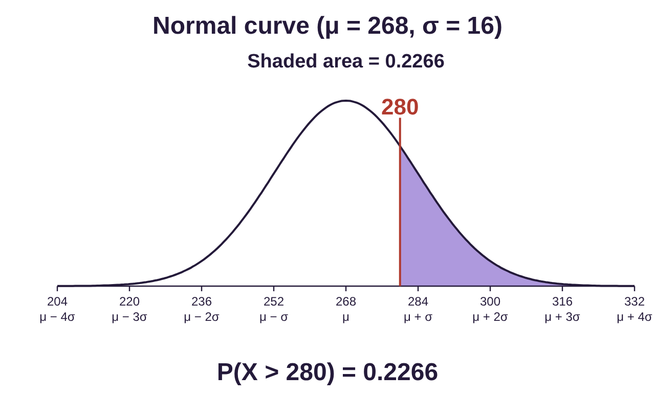
b)To find the probability that a pregnancy lasts longer than 280 days, we find $P(X>280)$. Choose “P(X > a)” and type 280 for the value a. We get $P\left(X>280\right)\approx 0.2266$. There is a 22.7% chance that a pregnancy will last at least 280 days. This is not unusual.

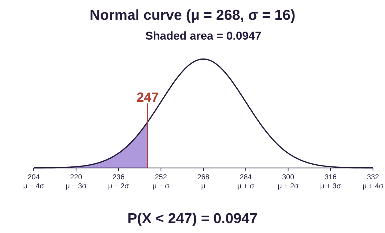
c)Three weeks early means 21 days before the mean, so the pregnancy would last fewer than 268 – 21 = 247 days. So, we find $P(X<247)$. Choose “P(X < a)” and type 247 for the value a. We get $P\left(X<247\right)\approx 0.0947$. Approximately 9.5% of pregnancies end with a preterm birth. This is not unusual.

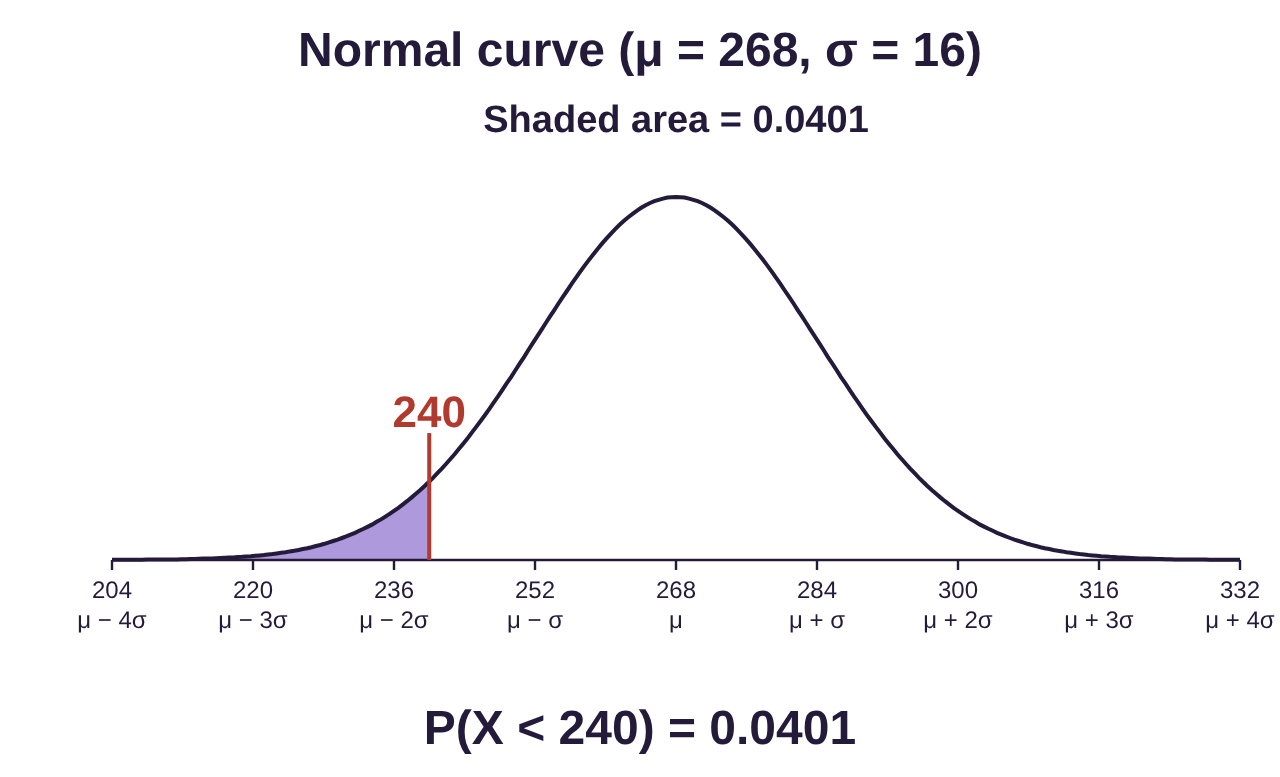
d)To find the probability a baby is born 4 or more weeks early, we subtract 28 days from the mean 268 – 28 = 240. We find $P\left(X<240\right)\approx 0.0401$. Approximately 4% of pregnancies end 4 or more weeks early. Since this is less than 5% chance, it would be unusual to have pregnancy end 4 or more weeks early.

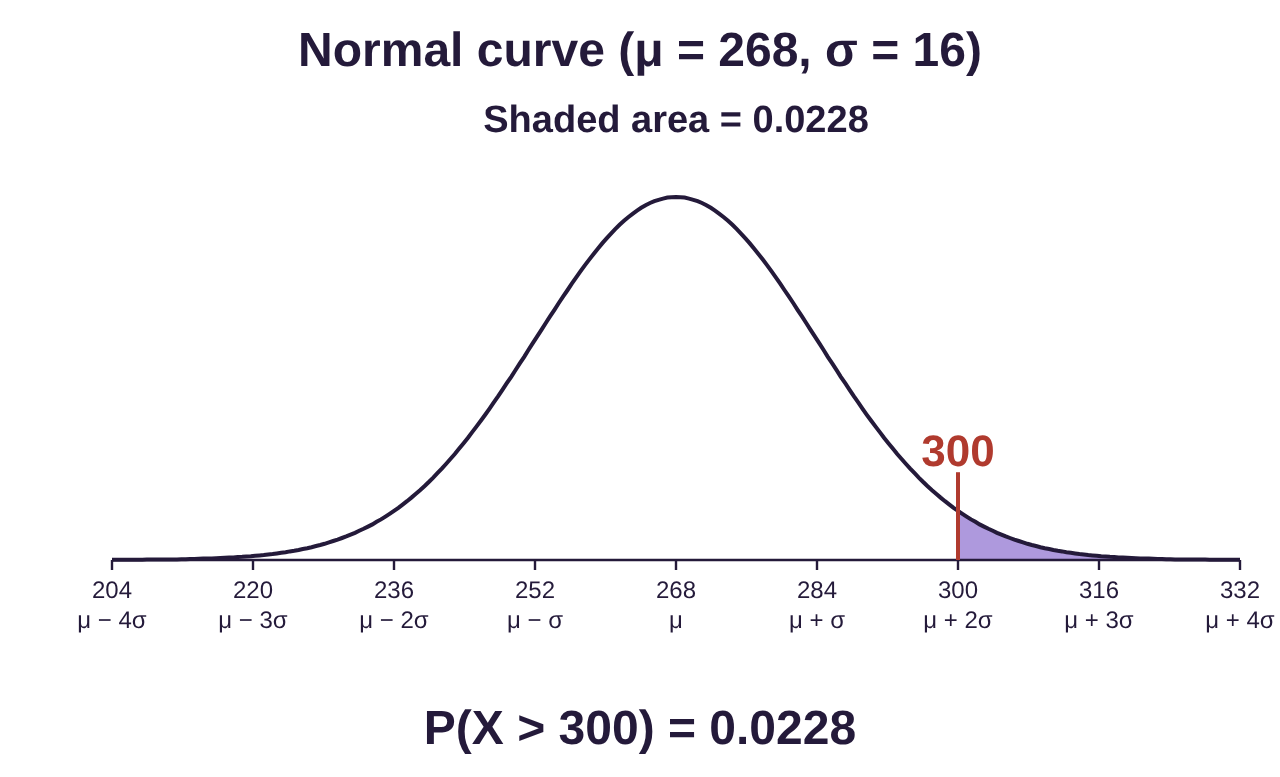
e)The probability that a pregnancy lasts 300 days or longer is $P\left(X>300\right)\approx 0.0228$. So, roughly 2.3% of pregnancies last at least this long. It is unusually long, but rare things happen!

Tip!

Solution:Open STATBELT Utility and select Calculators → Normal Calculator. Type in 8.2 for the mean and 0.12 for the standard deviation. Set “x-axis labels” to “Mean ± standard deviations” to show the mean and increments of the standard deviation.

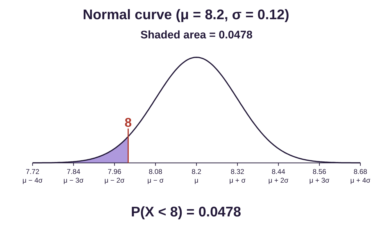
a)To find the probability that a chocolate bar weighs less than indicated on the package, we find $P(X<8)$. Choose “P(X < a)” and type 8 for the value a. The probability that a chocolate bar weighs less than 8 ounces is $P\left(X<8\right)\approx 0.0478$. Since this is less than 0.05 probability, a bar weighing less than 8 ounces is unusual.

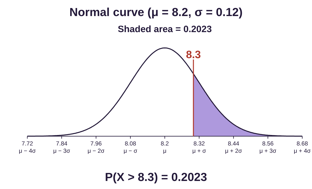
b)To find the probability that a chocolate bar weighs more than 8.3 ounces, we find $P(X>8.3)$. Choose “P(X > a)” and type 8.3 for the value a. The result is $P\left(X>8.3\right)\approx 0.2023$. About 20.2% of the chocolate bars weigh 8.3 or more ounces.

c)We want the machine to reject any bar that does not meet the minimum weight of 8 ounces. We also need it to filter out those that are too heavy, with weights above 8.5 ounces. So, a bar will be rejected either if it weighs less than 8 ounces OR more than 8.5 ounces. With these settings we can find the probability that a bar is rejected, and then convert that to a percent to answer the question.

We want to find $P\left(X<8\text{ OR }X>8.5\right)$. Remember that OR means we need to use the addition rule. Fortunately, the events $X<8$ and $X>8.5$ are disjoint (no chocolate bar weighs less than 8 ounces and weighs more than 8.5 ounces!) So, we can add the two probabilities together!

$$\begin{array}{cc}P\left(X<8\text{ OR }X>8.5\right)& =P\left(X<8\right)+P(X>8.5)\end{array}$$

We compute each of these probabilities separately, then add. We already found $P\left(X<8\right)\approx 0.0478$ in part (a). So, we need to find $P(X>8.5)$. In STATBELT, choose “P(X > a)” and type 8.5 for the value a. We get $P\left(X>8.5\right)\approx 0.0062$.

So finally,

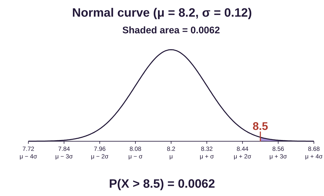
$$\begin{array}{cc}P\left(X<8\text{ OR }X>8.5\right)& =P\left(X<8\right)+P\left(X>8.5\right)\\ & \approx 0.0478+0.0062\\ & =0.054\end{array}$$

Based on this result, it appears that about 5.4% of chocolate bars are rejected due to being too small or too large.

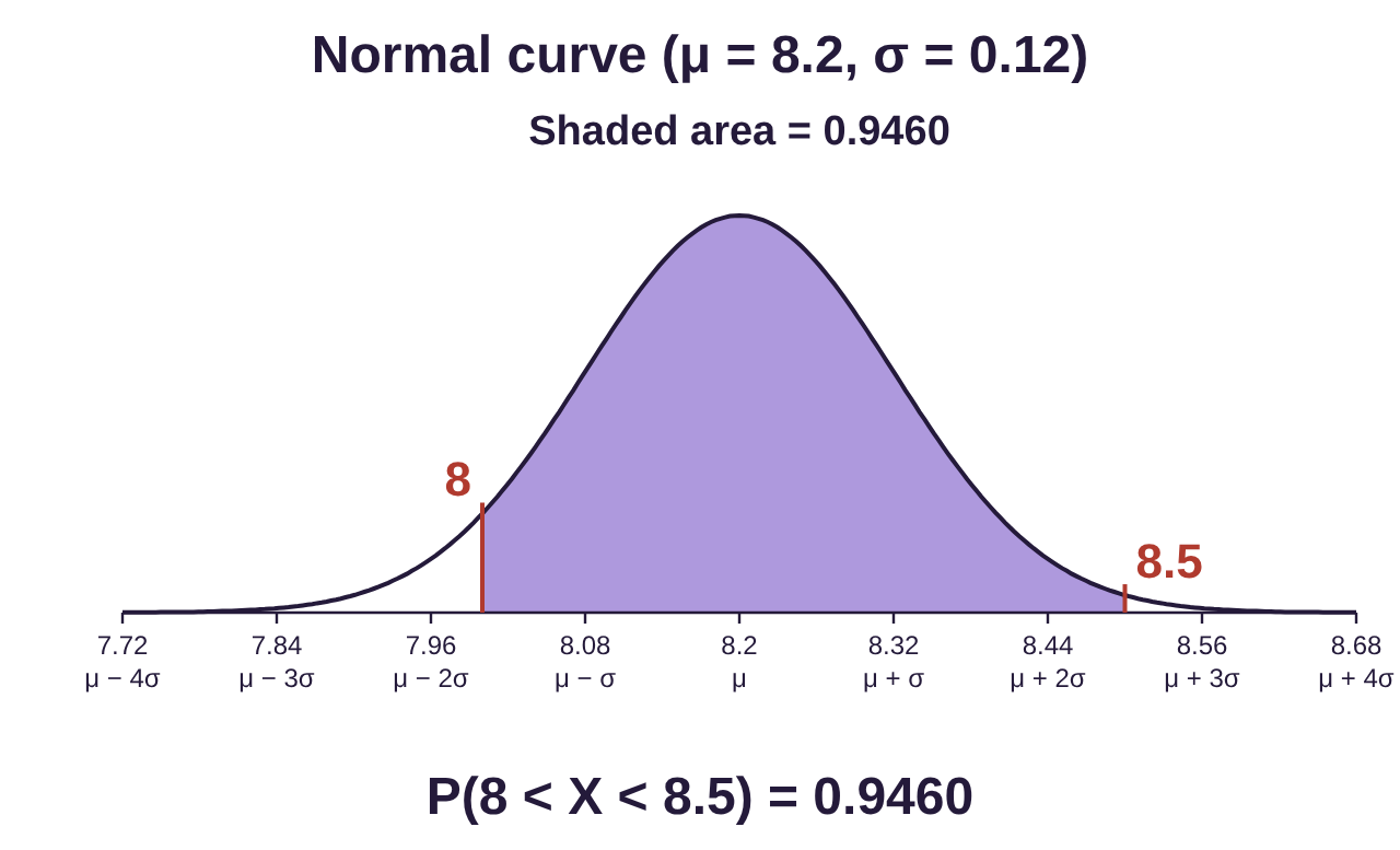
Note:Another way to compute $P\left(X<8\text{ OR }X>8.5\right)$ is to recognize that it is the complement of $P\left(8<X<8.5\right)$. If a chocolate bar is not lighter than 8 ounces, and not heavier than 8.5 ounces, then it must weigh somewhere between 8 and 8.5 ounces. If you recognize that, then $P\left(X<8\text{ OR }X>8.5\right)=1-P\left(8<X<8.5\right)$.

Choose “P(a < X < b)” and type 8 for the lower value a and 8.5 for the upper value b. The result is $P\left(8<X<8.5\right)\approx 0.9460$.

$$\begin{array}{cc}P\left(X<8\text{ OR }X>8.5\right)& =1-P\left(8<X<8.5\right)\\ & \approx 1-0.946\\ & =0.054\end{array}$$

In the picture at right, the unshaded area of the left and right tails, rather than the purple area in the middle, is the area representing the probability that we have found. STATBELT can also find this area directly: choose “P(X < a or X > b)” and type 8 and 8.5. The result is 0.0540.

Percentiles of the Normal Distribution

As you may recall, percentiles are used to describe position in a distribution.

Tip!

Percentiles always refer to the percent, probability, proportion, or area on the left! In probability language, that means we use $P(X\le a)$ when working with percentiles. See figure 7.19.

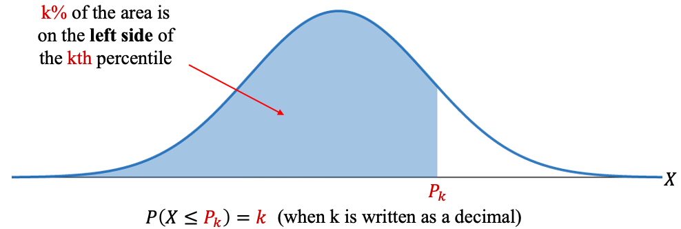
Figure 7.19: Percentiles always reference area on the left!

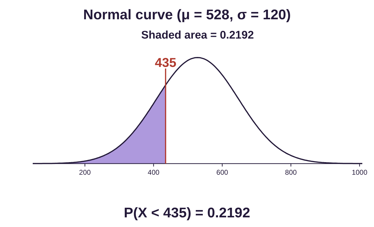
Solution:a)To find the percentile rank of 435, we need to know the percent of scores that are less than or equal to 435. We use the normal calculator with mean 528 and standard deviation 120. The proportion of area that is less than or equal to 435 is $P\left(X\le 435\right)\approx 0.2192$. We multiply this by 100 to make it a percent, $0.2192\times 100\%=21.92\%.$ We would say that Samuel scored at the 21^st percentile, because 21.9% of students scored less than or equal to his score. You might be tempted to round it up to 22%, but he did not score better than 22% of other students. He was almost at the 22^nd percentile, but not quite!

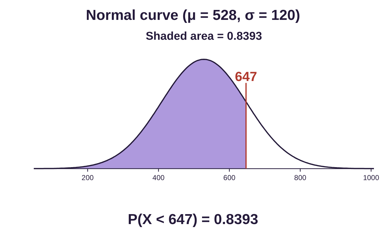
b)To find the percentile rank of 647, we need to know the percent of scores that are less than or equal to 647. Using STATBELT with the same mean and standard deviation gives us $P\left(X\le 647\right)\approx 0.8393$. We multiply this by 100 to make it a percent, $0.8393\times 100\%=83.9\%.$ We would say that Hercules scored at the 83^rd percentile, because 83% of students scored less than or equal to his score. The complement is that approximately 17% of students scored better than Hercules.

Solution:The 90^th percentile must have area = 0.9 on the left of the value for $X=P_{90}$. One way to find this is to use the Z-score that has area to the left equal to 0.9 to compute the raw score. Recall that the raw score is $X=\mu +Z\cdot \sigma$.

If we use the standard normal calculator, we can set the area to the left at 0.9. Under “Find a value from an area,” choose “P(Z < _) = a,” and type 0.9 for the area. See figure 7.20.

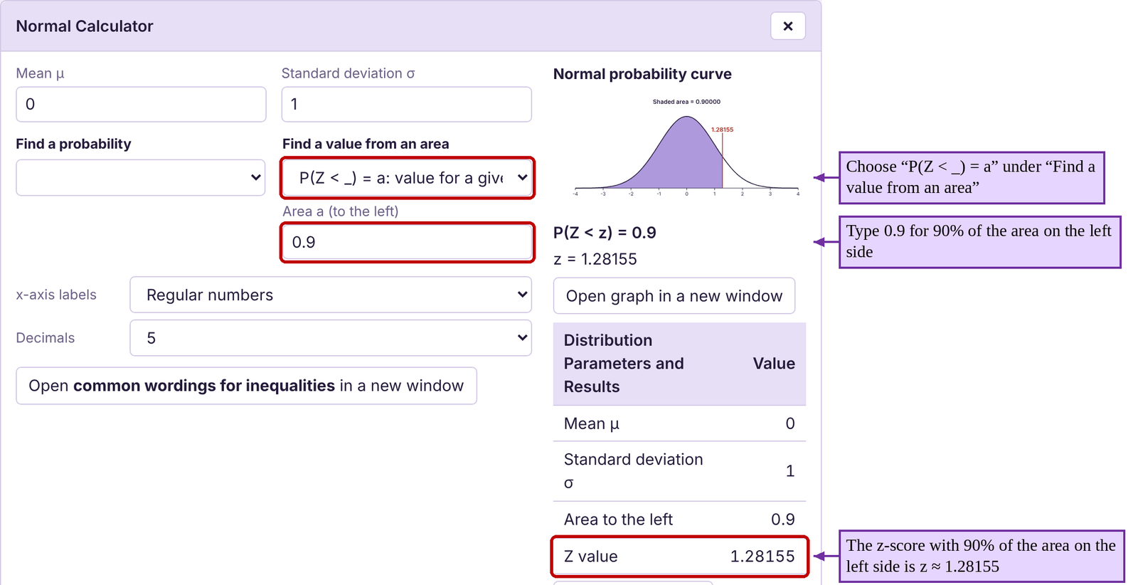
Figure 7.20: Using STATBELT to find a Z-score for a percentile.

The raw score that has $Z\approx 1.28155$ is $X=\mu +Z\cdot \sigma$

$$\begin{array}{cc}& =528+1.28155\times 120\\ & =528+153.786\\ & =681.786\\ & \approx 682\end{array}$$

So, a score of 682 represents the 90^th percentile of SAT Math scores on the 2020 exam.

Not all calculators have the following option, but STATBELT allows you to skip the previous work by inputting the mean and standard deviation directly, setting the area, and getting the raw score that represents the percentile. See figure 7.21 and the steps below.

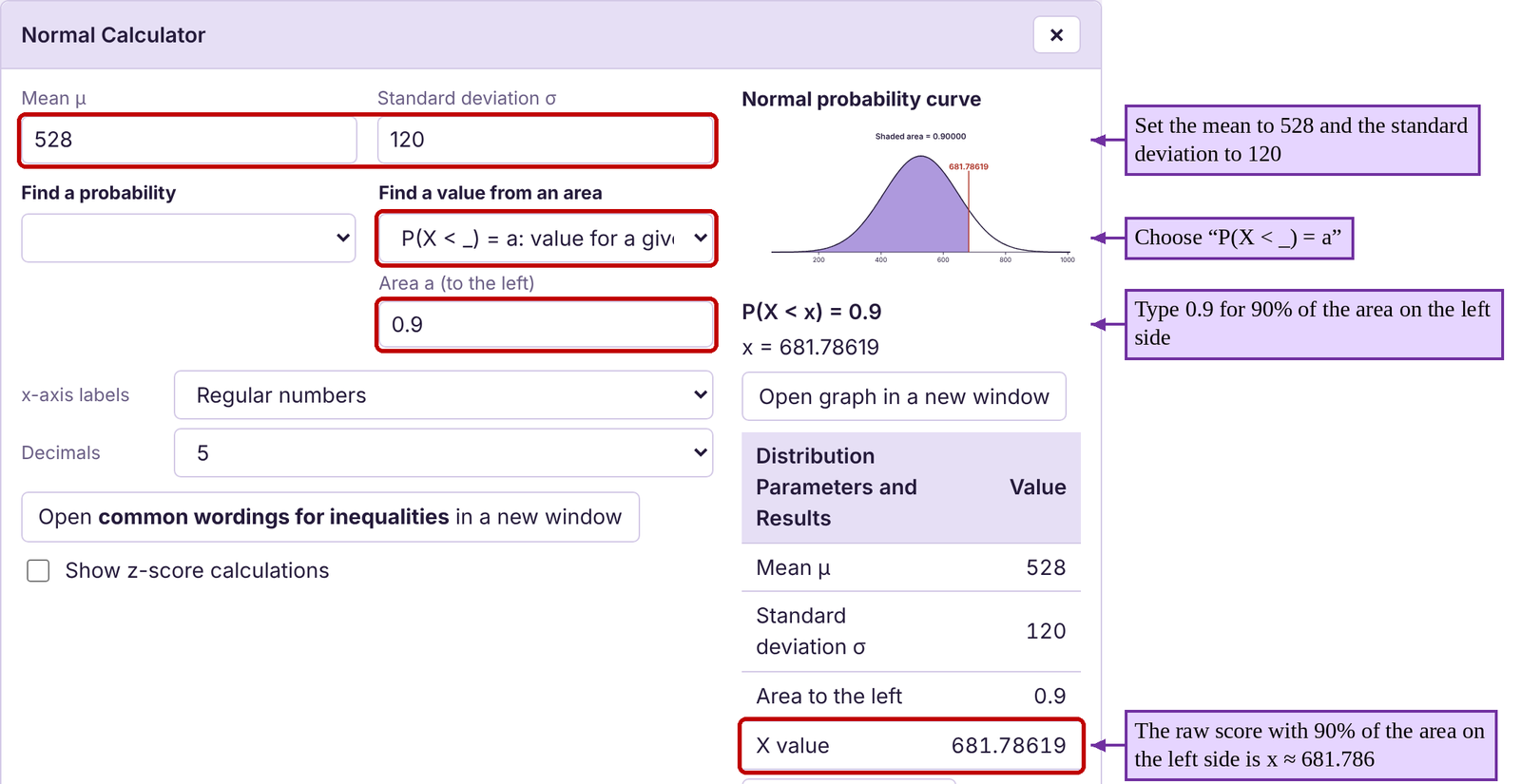
Figure 7.21: Using STATBELT to find a percentile.

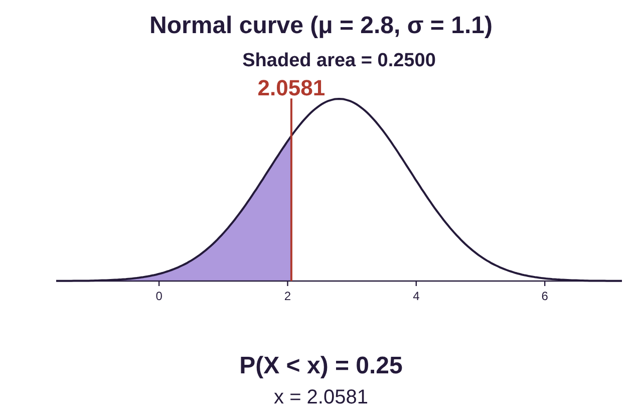
Solution:a)To find the 25^th percentile, select Calculators → Normal Calculator, and type in 2.8 for the mean and 1.1 for the standard deviation. Under “Find a value from an area,” choose “P(X < _) = a” and type 0.25 (the decimal equivalent of 25%) for the area. The 25^th percentile is $P_{25}\approx 2.06$ years, or approximately 24.7 months. About 25% of cell phones will be replaced prior to reaching 2.06 years of use.

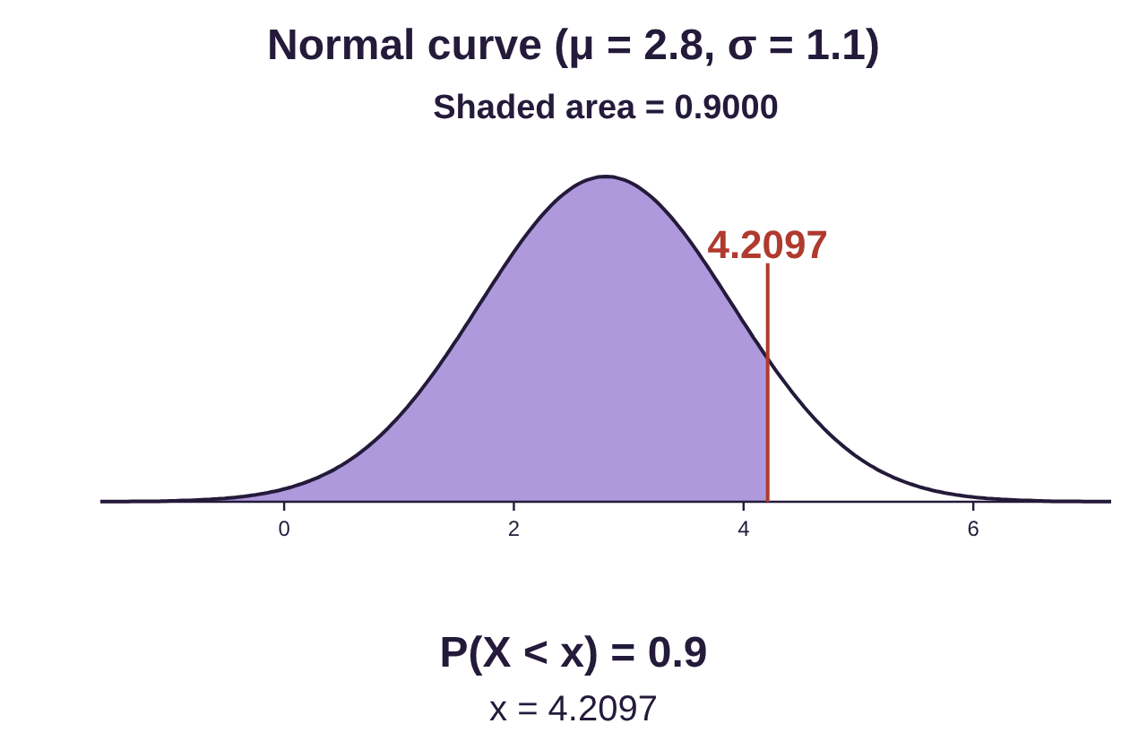
b)To find the 90^th percentile, repeat the steps in part (a) and type 0.9 (the decimal equivalent of 90%) for the area. The 90^th percentile is $P_{90}\approx 4.2$ years, or approximately 50.4 months. About 90% of cell phones will be replaced prior to reaching 4.2 years of use.

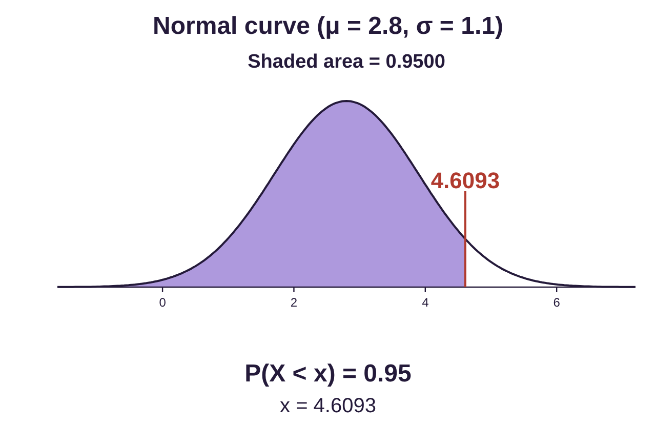
c)To find the cutoff for the top 5% of lifespans, we must first realize that this is the same as the 95^th percentile. Remember that $P_{95}$ is the value such that approximately 95% is lower and approximately 5% is higher. So, type 0.95 for the area. The 95^th percentile is $P_{95}\approx 4.6$ years. So, about 5% of cell phones will last longer than 4.6 years.

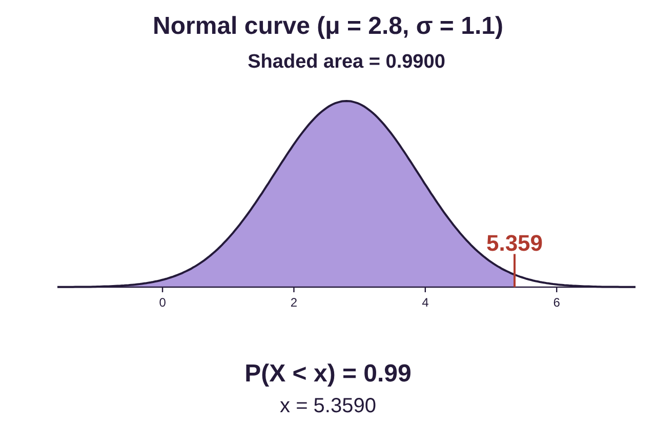
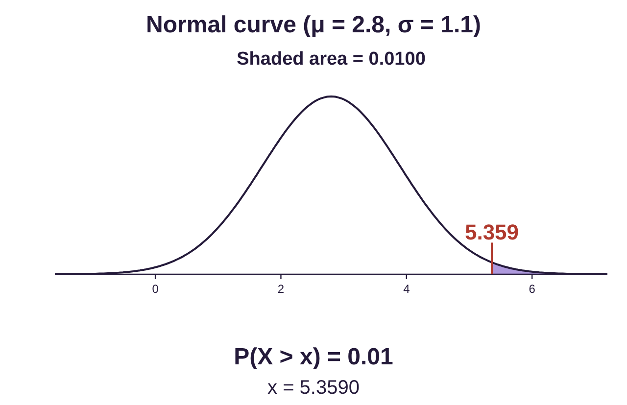
d)To identify the lifespan that determines the top 1% of cell phones, we must recognize that this is the same as the 99^th percentile. Approximately 99% of phones are replaced before $P_{99}$ while about 1% last longer than $P_{99}.$ Type in 0.99 for the area. The 99^th percentile is $P_{99}\approx 5.36$ years. About 1% of cell phones will last longer than 5.36 years before being replaced, while 99% will be replaced before reaching 5.36 years old.

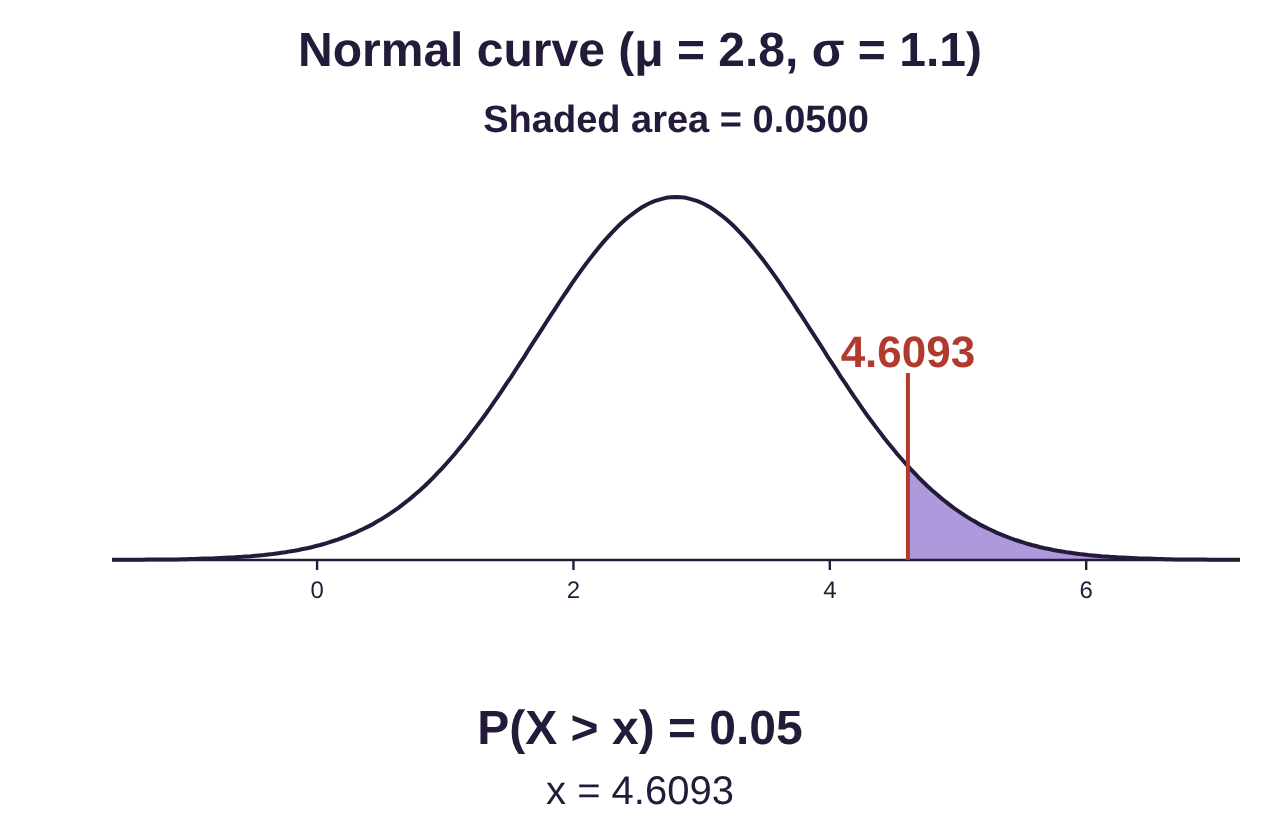
If you are wondering, there is another way to complete parts (c) and (d) in example 9. For part (c), we want to identify the top 5%. We can choose “P(X > _) = a” and set the area to 0.05. The graph looks different, with the shaded region in the right side tail rather than on the left. The right side is the “top” in this sense, and the left side is the “bottom.” But you will notice that the X value is the same, both equal to 4.609 years. Not all calculators can do this, so it is good to know both approaches.

Similarly, if you want to find the top 1%, you can choose “P(X > _) = a” and set the area to 0.01. STATBELT shades the right tail as the top 1%, with the cut off at 5.36. These are examples of right tail probabilities. We will use tail probabilities in the next few chapters when we study inference.

Tip!

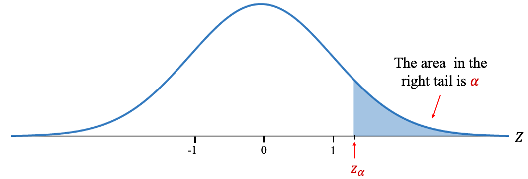
Figure 7.22: Illustration of the definition of $z_{\alpha }$.

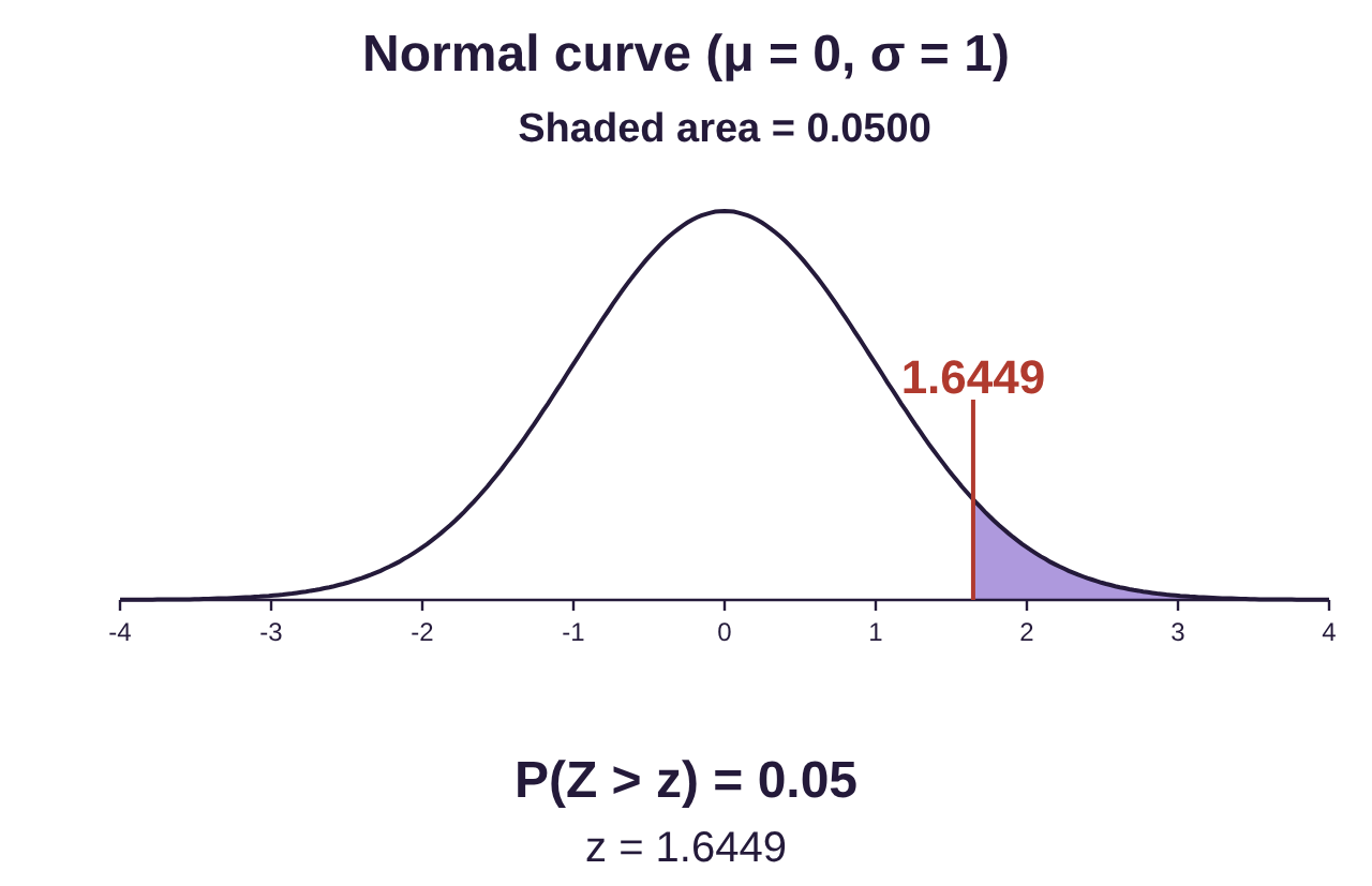
a)To find $z_{\alpha }=z_{0.05}$, open the normal calculator (Calculators → Normal Calculator), choose “P(Z > _) = a” under “Find a value from an area,” and type 0.05 for the area. The result is $z_{0.05}\approx 1.645$. The interpretation is that about a 5% of the values from a standardized normal variable would be above 1.645. So, an observation from a normal distribution with a z-score above 1.645 would be considered unusual.

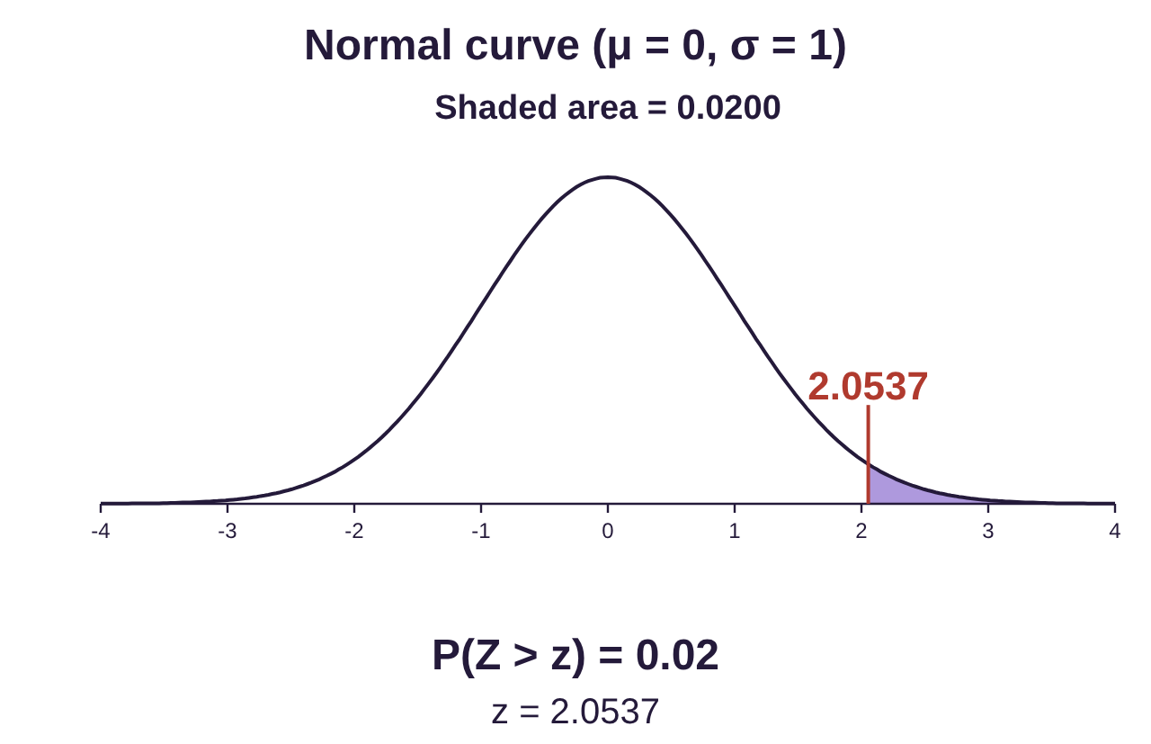
b)To find $z_{\alpha }=z_{0.02}$, leave “P(Z > _) = a” chosen and type 0.02 for the area. The result is $z_{0.02}\approx 2.054$. Approximately 2% of standard normal values are higher than 2.054. If X is a normal random variable, about 2% of X values will have z-scores that are higher than 2.054. An observation with a z-score above 2.054 would be unusual.

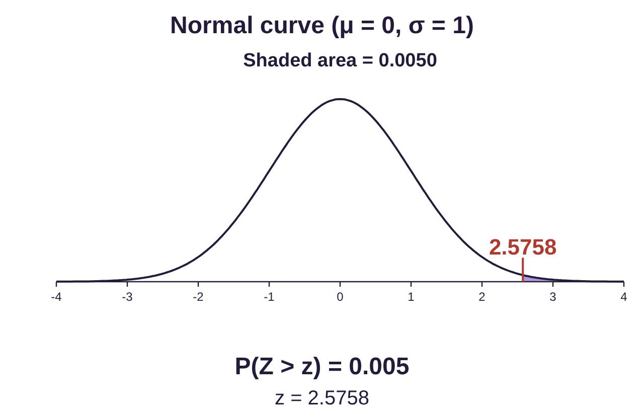
c)To find $z_{\alpha }=z_{0.005}$, type 0.005 for the area. The result is $z_{0.005}\approx 2.576$. Only 0.5% (one-half of one percent) of standard normal values are higher than 2.576. Any observation that has a z-score that is higher than 2.576 is very unusual!